Assortment and Cut of Defective Stocks by Bilevel Programming

Claudio Arbib

1 a

, Fabrizio Marinelli

, Mustafa C¸ . Pınar

and Andrea Pizzuti

Dipartimento di Ingegneria/Scienze dell’Informazione e Matematica, Universit

a degli Studi dell’Aquila, L’Aquila, Italy

Dipartimento di Ingegneria dell’Informazione, Universit

a Politecnica delle Marche, Ancona, Italy

Department of Industrial Engineering, Bilkent University, Ankara, Turkey

Keywords:

Assortment Problem, Cutting Stock Problem, Defects, Bilevel Programming.

Abstract:

In this paper we deal with the problem of deciding the best assortment and cut of defective bidimensional

stocks. The problem, originating in a glass manufacturing process, can arise in various industrial contexts. We

propose a novel bilevel programming approach describing a competition between two decision makers with

contrasting objectives: one aims at fulﬁlling production requirements, the other at generating defects that,

damaging the products, reduce yield as much as possible. By exploiting nice properties of adversarial optimal

solutions, the bilevel program is rewritten as a one-level 0-1 linear program. Computational results achieved

on random instances with realistic features are discussed, showing the quality and the beneﬁts of the proposed

approach in reducing the yield loss from defective material in a worst-case perspective.

1 INTRODUCTION

This study ﬁnds its initial motivation in the optimiza-

tion of a ﬂoat glass manufacturing process. A pro-

cess of this type is organized in two main stages. The

ﬁrst employs a ﬂoat furnace to produce large rectan-

gular glass sheets (large items): these are obtained

in various measures, ranging from 12.6 to 19.6 sqm,

by widening/narrowing a ribbon of molten glass, and

then sent to warehouse. In the second stage, small

rectangular sheets (small items), sizing between 0.21

and 3.3 sqm, are cut from the large ones previously

manufactured, and then sent to downstream depart-

ments.

Mathematical programming models (Arbib and

Marinelli, 2007; Arbib and Marinelli, 2009) were

originally designed (and assessed in practice) for the

simultaneous optimization of large sheet assortment

and cut in the above-mentioned process. The assort-

ment issue refers to the number of distinct large sizes

stored in the warehouse at any time: this number (po-

tentially large up to 6500) must be limited to a certain

amount p (typically ≤ 20) so as to contain holding

cost and setups, and also to facilitate handling oper-

ations. The cutting issue requires on the other hand

to fulﬁll a known demand of distinct small sizes. The

minimization of the trim loss, i.e., the difference be-

tween the total area of used glass and the total area of

https://orcid.org/0000-0002-0866-3795

required small parts, is sought on the whole.

The two quoted papers study the problem in a de-

terministic context, assuming perfect knowledge of

all the necessary data. However, glass fabrication nat-

urally carries the burden of imperfections (e.g. bub-

bles) that, occurring in a substantially unpredictable

way, may compromise the quality of small items and

hence reduce yield. The estimated loss due to de-

fects is a non-negligible cost term, sometimes even

larger than trim loss. This, in the end, motivated

us to investigate ways to model and compute defect-

reconﬁgurable cutting patterns.

Approaching the issue of faultiness, one can ei-

ther assume an a-priori knowledge of defect posi-

tions in raw material (as in most literature), or cap-

ture the stochastic nature of defects by modeling

their occurrence as a random process which gener-

ates faults in the large items. The approach which

best ﬁts the observed situation depends on both prac-

tical and problem-speciﬁc elements. In our case, no

prior knowledge of defects is available before the end

of large items fabrication in the ﬁrst stage. In addi-

tion, the decision process simultaneously deﬁnes both

large items assortment and cutting patterns, and there-

fore penalizes on-line strategies in which defect-free

patterns are redesigned after spotting the faults. This

policy would in fact completely consume the yield

gain with additional material handling, machine se-

tups and operation scheduling for downstream depart-

294

Arbib, C., Marinelli, F., Pínar, M. and Pizzuti, A.

Assortment and Cut of Defective Stocks by Bilevel Programming.

DOI: 10.5220/0010896600003117

In Proceedings of the 11th International Conference on Operations Research and Enterprise Systems (ICORES 2022), pages 294-301

ISBN: 978-989-758-548-7; ISSN: 2184-4372

ments.

In practice, though imperfections are spotted by

visual inspection and marked on the large items, they

are not considered before the cutting stage, and small

items affected by faults are simply discarded before

the following stages of the production process. Mod-

elling problem uncertainty is therefore preferable and,

in any case, is a step beyond the straightforward reac-

tion of just reckoning defects at the end of the cutting

stage, and then simply discard faulty items.

That said, a production policy in presence of de-

fects is liable of two complementary visions: (i) pri-

oritize demand fulﬁllment (as in just-in-time philos-

ophy) and overproduce minimizing the need of raw

material; (ii) given some availability of raw mate-

rial, maximize the expected faultless production on

can obtain from it, covering possible order backlog

by safety stocks.

Policy (i) was addressed in (Arbib et al., 2021).

In this paper we follow policy (ii) and deﬁne a novel

bilevel mathematical formulation of an assortment-

and-cut problem to maximize the total value of fault-

less small item production: defect occurrence is mod-

eled as an optimization problem solved by an adver-

sarial follower that tries to place defects in a way

that reduces production value as much as possible.

The worst-case perspective of the adversarial model

is subject to the following assumptions:

• the adversary can place at most one defect at ran-

dom in each large item;

• the total number of defects the adversary can place

in the planning horizon is a model parameter;

• yield reduction is measured by the expected value

of small item loss, computed in turn by the proba-

bility that no cut reconﬁguration exists, which al-

lows defect avoidance.

The ﬁrst of these assumptions is indeed quite restric-

tive, yet is compliant with some real productive pro-

cesses, where defects are sufﬁciently spread on raw

material, i.e., where defects do not form clusters and

rather appear according to a spatial Poisson point pro-

cess. Moreover, it help us give a ﬁrst clear formaliza-

tion in bilevel terms under mild hypothesis, indicat-

ing an original robust optimization methodology to be

hopefully extended in the future.

2 LITERATURE REVIEW

Since the seminal paper of Gilmore and Gomory

(Gilmore and Gomory, 1961), a vast amount of scien-

tiﬁc contributions were dedicated to cut optimization,

focusing on both the theoretical and practical side of

the problem, see (W

ascher et al., 2007). Although

cutting problems with defects were considered very

early (Hahn, 1965), quite few papers address this is-

sue. Most contributions assume defect sizes and lo-

cations known in advance: to quote just an example,

(Aboudi and Barcia, 1998) study the MINIMUM DE-

FECTIVE SUBSET SUM which asks to ﬁnd a new pat-

tern layout avoiding the largest possible number of

defects in a one-dimensional stock. To the best our

knowledge, only (Sculli, 1981) and (Ghodsi and Sas-

sani, 2005) consider instead stochastic settings. In the

former, to handle fringe defects in insulating tape pro-

duction, roll size is treated as a normal random vari-

able that models damages caused by winding. The lat-

ter addresses a real-time wood cutting process where

each strip to be cut is subject to random variations of

quality along its length.

Due to the wide range of manufacturing contexts

where cutting is involved, the theme of defectiveness

is characterized by a multiplicity of features: holes

and stains in leather or paper sheets, bubbles in glass,

knotholes in wooden boards. This variety originated a

corresponding richness of defect models, from point-

shaped to convex areas, from imperfections compro-

mising the quality at various grades to faults com-

pletely ruining the items.

In (Carnieri et al., 1993) a two-stage deci-

sion model is proposed for application in a one-

dimensional lumber cutting problem, in which each

stock item is affected by a single defect. Under the

same restriction of one defect per stock item, (Nei-

dlein et al., 2009) address a two-dimensional cutting

problem and propose an AND/OR-graph approach for

the defective case.

Multiple defects per stock item are also consid-

ered. In (Ozdamar, 2000) a concurrent scrap min-

imization/proﬁt maximization one-dimensional tex-

tile cutting problem is discussed and dealt with, us-

ing a mutative simulated annealing. A genetic algo-

rithm is presented by (Wenshu et al., 2015) for cutting

one-dimensional wood board with possibly decayed

portions, which affect product appearance and mate-

rial strength. In a two-dimensional setting, (Afshar-

ian et al., 2014) investigate a dynamic programming-

based heuristic that aims at maximizing the value of

the small items produced.

Among papers that consider product values con-

ditioned to stock faults, (Sarker, 1988) studies the op-

timal use of defect-free areas and devises a dynamic

programming procedure for the maximization of to-

tal sales value. Similarly, (R

onnqvist and

Astrand,

1998) optimize a wood-board cross cutting process

by a mathematical formulation and dynamic program-

ming. Finally, (Durak and T

un, 2017) presents an

Assortment and Cut of Defective Stocks by Bilevel Programming

295

on-line optimization setting in glass manufacturing

where the ﬂoat line is directly equipped with sensors:

hence, cutting patterns can be redeﬁned on the ﬂy to

avoid defects, but only within few seconds after de-

tection and according to several physical constraints

that limit pattern conﬁgurations. Solutions are com-

puted by dynamic programming and MILP-based al-

gorithms. To the best of our knowledge, no reference

addresses the combined assortment-and-cut problem

discussed here.

3 THE ASSORTMENT-AND-CUT

PROBLEM

In this section we brieﬂy review the 0-1 Linear Pro-

gram presented in (Arbib and Marinelli, 2009) to

model an assortment-and-cut problem arising in a real

manufacturing plant.

Technical constraints of the cutting machines and

organizational rules imposed by the management im-

pose several restrictions to cutting patterns:

• Only guillotine cuts are admitted, the ﬁrst one al-

ways horizontal.

• A large item can only be cut into single-size

equally oriented small items (always choosing the

most productive item orientation).

• Cutting patterns are built from top-left, hance trim

loss is always positioned at the bottom-right cor-

ner of the large item.

Let L (let S) be the set of all feasible large (of re-

quired small) sizes that can be produced in the ﬁrst

(second) stage. Let W

and H

and h

) respec-

tively be the width and height of j ∈ L (of i ∈ S) and

= W

= w

) be the item area. Suppose also

i ∈ S required in d

copies in the planning horizon.

The demand d

can be fulﬁlled by cutting an arbi-

trary subset P ⊆ L of large sizes. For each j ∈ P, up

to n

i j

= bA

c small items of size i can be obtained

from a large item of size j (we say that n

i j

is the out-

come of a maximal cutting pattern). Introducing the

integer variable y

i j

≥ 0 to count how many large items

j are employed to manufacture small size i, the total

material cost c

to cut i from j ∈ P can be computed

through the following integer knapsack problem:

= min

∑

j∈P

i j

(1)

∑

j∈P

i j

≥ d

i j

∈ Z

Costs c

are then plugged into the following

mathematical model of the assortment-and-cut prob-

lem:

min

∑

i∈S

∑

P⊆L

(2)

∑

P⊆L

= 1 i ∈ S (3)

∑

P⊆L:P3 j

≤ z

i ∈ S, j ∈ L (4)

∑

j∈L

≤ p (5)

, z

∈ Z

i ∈ S, j ∈ L,P ⊆ L

The x

and z

are implicitly forced to behave as

binary variables in the model. Hence, we interpret

= 1 if the whole demand of small size i is met by

cutting large sizes j ∈ P, and z

= 1 if at least one

large item of size j ∈ L is cut.

The objective function measures the total amount

of glass employed in the process. Equations (3) en-

sure demand fulﬁllment for all i ∈ S; inequalities (4)

identify the distinct large sizes j ∈ L selected in the

assortment from subsets P ⊆ L; ﬁnally, by (5), the as-

sortment must not exceed p different sizes.

Since variables x

are exponentially many in the

cardinality of L (i.e. O(|L|)

), (Arbib and Marinelli,

2009) solve (2) by column generation. A very effec-

tive heuristic can anyway be devised by restricting

subsets P to singletons { j}, so that each small size

i is produced by only one large size in L. This brings

to a p-median formulation that widely shrinks the size

of (2) and well approximates the original problem, as

its optimal value asymptotically tends to the true opti-

mum as small item requirements increase (Arbib and

Marinelli, 2009). Note, in particular, that for P = { j}

the optimal solution of (1) is immediately found as

¯y

i j

, min{y

i j

: n

i j

≥ d

i j

∈ Z

} = d

i j

e (6)

which gives the number of large items of size j satu-

rated to fulﬁl the entire demand of small sizes i.

The nice properties of the p-median formulation

allow us to refer from now on to this simpliﬁed model,

that we will use as starting point for the design of our

bilevel approach. The model can however be gener-

alized to non-singleton sets by an appropriate change

of variables.

4 BILEVEL MODEL

Bilevel programming provides a mathematical model

of Stackelberg games. These are strategic games de-

scribing the sequential interaction of two players: a

ICORES 2022 - 11th International Conference on Operations Research and Enterprise Systems

296

leader, or upper-level player, and a follower, or lower-

level player. The leader makes decisions assuming

that the follower will react in a rationally optimal way.

For an introduction to bilevel optimization, see the

survey by (Colson et al., 2005).

Our bilevel framework entails two decision mak-

ers D

that compete with contrasting goals: D

aims at the best usage of material to fulﬁll demand;

, the adversary, tries to impair it as much as pos-

sible by distributing f defects in the large items to-

tally produced by D

, at most one per large item. As

said, we illustrate the model assuming that D

uses

the approximated version of the assortment-and-cut

problem described in §3, with variables x

deﬁned

for singletons only.

Let us consider the solutions of (2)-(5) that main-

tain the total requirement of raw material under a pre-

scribed supply A

. For any i ∈ S, j ∈ L, let then x

i j

= 1

if and only if large size j is used to produce the whole

demand of item size i. A pair (i, j) ∈ S × L for which

i j

= 1 will be called from now on a production.

For sufﬁciently large A

, the following system has

a solution that represents a set of productions that ful-

ﬁll the whole demand:

)

∑

j∈L

i j

= 1 i ∈ S (7)

∑

i∈S

∑

j∈L

i j

≤ A

(8)

i j

≤ z

i ∈ S, j ∈ L

∑

j∈L

≤ p

i j

, z

∈ Z

i ∈ S, j ∈ L

where c

i j

is the optimum value of (1) for P = { j}. All

such solutions have the same total value

∑

i∈S

where a

is the area of (or perhaps the economical

value attributed to) each item of size i ∈ S.

The decision of D

is encoded by variables u

i j

∈

IN that indicate the number of large items j that con-

tain a defect and are cut to obtain item size i. Let ˜x be

a particular feasible solution to (D

) and π

i j

denote

the probability of existence of a faulty item of size i

from a single large item of size j (this probability will

be computed in §5). With these positions, the largest

return of the adversarial choice is obtained by solving

the following ILP:

) max

λ( ˜x,u) =

∑

i∈S

∑

j∈L

i j

(9)

∑

i∈S

∑

j∈L

i j

≤ f

i j

≤ ¯y

i j

˜x

i j

i ∈ S, j ∈ L

i j

∈ Z

i ∈ S, j ∈ L.

with the ¯y

i j

given by (6). The objective function is

the expected loss of D

, that is the expected value of

small items lost when at most f large items are hit by

a defect. The total amount of defects distributed by

is bounded by the ﬁrst inequality, while the sub-

sequent bounds ensure that no more large items than

those used in production j can be affected by a fault.

Problem (D

) is a continuous knapsack with

bounded variables, therefore an optimum to (9) can be

found in O(nlog(n)) time by initially ranking produc-

tions (i, j) in non-increasing order of weighted losses

i j

, then sequentially saturating bounds by setting

i j

= ¯y

i j

˜x

i j

while

∑

i∈S

∑

j∈L

i j

≤ f

and placing the unsaturated difference to f defects (if

any) on the production with the largest of the remain-

ing loss.

More interestingly, this helps us build a compact

formulation of the bilevel problem

max

x∈D

− max

x∈D

,z∈D

λ(x,u)} (10)

By the above argumentation, for i,h ∈ S and j,k ∈

L such that (i, j) ≺ (h, k), u

> 0 implies u

i j

= ˜x

i j

whereas u

= 0 implies u

i j

≤ ˜x

i j

. We can write those

conditions by suitable linear inequalities, so formulat-

ing the bilevel problem (10) as a one-level 0-1 LP:

(BP) min

∑

i∈S

∑

j∈L

¯y

i j

(11)

subject to D

and:

i j

+ η

− η

i j

≤ 1 (i, j) ≺ (h,k) (12)

i j

− x

i j

≤ 0 i ∈ S, j ∈ L (13)

∑

i∈S

∑

j∈L

¯y

i j

≥ f (14)

i j

∈ {0,1} i ∈ S, j ∈ L

where η

i j

= 1 if and only if production (i, j) is faulty.

The objective function (11) is the same as (9) and

represents the largest loss D

can impose to any feasi-

ble choice of D

. Inequalities (12) impose the dis-

cussed ranking condition: assuming (i, j) ≺ (h,k),

if the (i, j)-th production is chosen and the (h,k)-th

production is affected by defects, then the (i, j)-th

production must have faults. Inequalities (13) state

Assortment and Cut of Defective Stocks by Bilevel Programming

297

on one hand that a production not chosen cannot of

course be faulty; on the other hand, if it is faulty, then

it must be chosen and the number of its faults must

be ¯y

i j

. Finally, inequality (14) enforces D

to insert at

least f defects: minimization will then reduce faults

to the smallest possible amount.

An optimal solution to model (BP) may not be re-

ally optimal: the problem arises when (14) is fulﬁlled

with the sign >. To cope with this inconvenience, it

is necessary to allow the last nonzero variable η

i j

the ranking to get values between 0 and 1. However,

we do not know in advance which variable will be the

last in the ranking induced by an optimal solution, so

we have to identify it using the differences between

consecutive η

i j

. We then introduce real variables θ

i j

that optimization will set all to 0 but one, ﬁxed to the

surplus value

∑

h,k

¯y

− f . The new variables obey

0 ≤ θ

i j

≤ ¯y

i j

i ∈ S, j ∈ L

i j

≤ ¯y

i j

(1 − η

) (i, j) ≺ (h,k)

i j

≤

∑

h∈S

∑

k∈L

¯y

− f i ∈ S, j ∈ L

The former constraints allow just one nonzero,

precisely the θ

i j

associated with the last η

i j

> 0 in

the ranking; the latter constraint allows it to get up to

the correct surplus. Optimization will then set it to the

exact surplus as soon as we subtract the term

g =

∑

i∈S

∑

j∈L

i j

from the objective function.

Passing to variables x

, one can rewrite (D

) as in

(2), maintaining the objective function (11) and con-

straints (12), (13) in the x

i j

variables, and adding the

inequalities

− x

i j

≤ 0 i ∈ S, j ∈ P (15)

In this case, for j ∈ P the ¯y

i j

form an optimal so-

lution of (1) — note that if ¯y

i j

= 0 then j can be re-

moved from P, thus implications (15) hold only for

active productions.

Note also that the number of constraints (15)

grows linearly with the cardinality of S and P, but

recall that in principle the x

variables are exponen-

tially many. A formulation that avoids such a large

number of constraints (and the consequent row gener-

ation) can however be devised rewriting inequalities

(12), (13) as

+ η

− η

i j

≤ 1 j ∈ P,(i, j) ≺ (h,k) (16)

i j

−

∑

P3 j

i j

≤ 0 i ∈ S, j ∈ P

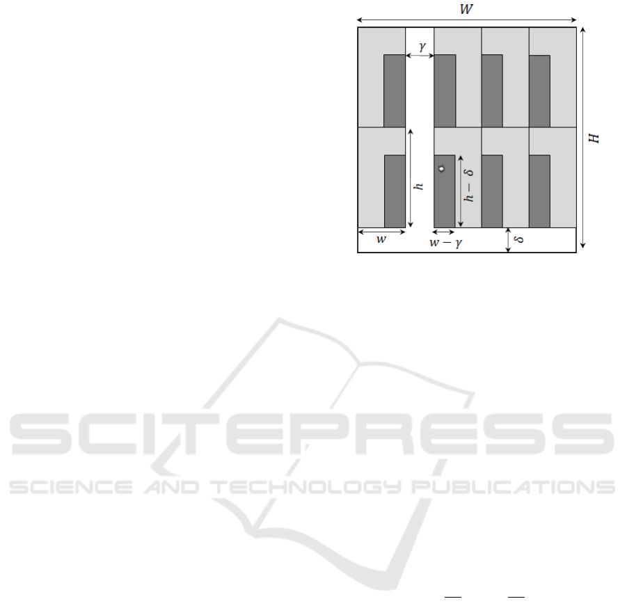
Figure 1: A defect falling in a vertical or horizontal strip

(white) can be recovered; a defect in the critical area (dark

grey rectangles) causes the loss of one item.

5 FAULT MODEL

The cost coefﬁcients c

i j

in (7), that one computes by

(1), are uncertain due to defects that may alter the

value of parameters n

i j

. Suppose those defects point-

shaped, statistically independent and uniformly dis-

tributed in A

(which, we recall, is an amount of ﬂoat

material sufﬁcient to meet the whole small item re-

quirement: a lower estimate of A

∑

, a more

reﬁned evaluation can be found solving problem (2)).

Given an evaluation of A

and an upper bound f

to the total number of faults that can affect the entire

ﬂoat campaign, the probability that the j-th size of L

exhibits a defect is

= f





1 −



f −1

However, the yield reduction consequent to faults is

also dependent on both where the defect falls in the

large item and which small item is cut from that item.

We consider the most general case in which pattern

layouts can be freely reconﬁgured, also by splitting

waste strips with additional cuts, and will call critical

a defect that causes a small item loss for any admis-

sible reconﬁguration of the pattern layout. For any

production (i, j), κ

i j

is then the probability that a sin-

gle large item of size j used for manufacturing small

items of size i has a critical defect. Clearly, κ

i j

= 0

if the pattern is non-maximal. To illustrate its com-

putation, we refer to Figure (1) and temporarily drop

indices i ∈ S and j ∈ L.

Let us assume a large item of unitary area A = 1

from which small items are cut. Let moreover α =

ICORES 2022 - 11th International Conference on Operations Research and Enterprise Systems

298

c and β = b

c respectively count the columns and

rows in which small items are aligned in the pattern.

Packing all items according to a top-left strat-

egy leaves two overlapping strips: one horizontal, of

height δ = H − βh and area δW , at the bottom of the

large item; and one vertical, of width γ = W − αw

and area γH, to its extreme right. Similarly, strips

of the same size can be obtained by aligning part of

the α small item columns (part of the β rows) to the

extreme right (respectively, the bottom) of the large

item. Any such re-alignment is a pattern reconﬁgu-

ration that avoids a defect falling in the strips, so any

such defect is non-critical.

Instead, there exists a critical area complementary

to that covered by the above strips such that a defect

falling in it will surely compromise an item, what-

ever the pattern layout. This critical area consists of

the black identical rectangles displayed in Figure (1),

which are αβ and have width w − γ and height h − δ.

Hence, by construction

κ = αβ(w − γ)(h − δ)

For non-unitary large items the above formula is im-

mediately adapted by normalizing w,γ with respect to

W , and h, δ with respect to H.

Finally, the probability π

i j

that a large item in pro-

duction (i, j) has a critical defect is given by the com-

pound probability ϕ

i j

6 NUMERICAL TESTS

We did some numerical tests using an Intel

Core

i7-7500U (2 cores) 2.90 GHz with 16Gb RAM. Math-

ematical formulations were implemented with AMPL

and solved by IBM

CPLEX

12.9.0.0 with default

setting and a time limit of 600 seconds.

Experiments aim at assessing usability and bene-

ﬁts of formulation (BP) as a tool to evaluate the worst-

case yield loss induced by material defectiveness. We

discuss a comparison with the solutions obtained via

the p-median approximation of (2), with worst-case

loss measured by running the adversarial model D

with ˜x taken from the computed solutions.

Tests were made on a set of 200 randomly gen-

erated instances of limited dimensions, divided into

8 groups of 25 instances according to combinations

of the number of small sizes |S| ∈ {5,6, 7,8} and the

assortment level p ∈ {|S| − 1,|S| − 2}. Compliantly

with the production features described in (Arbib and

Marinelli, 2007), we assumed large sizes (in meters)

∈ [2.80, 3.21] and H

∈ [4.50, 6.10] for j ∈ L, small

sizes i ∈ S randomly generated as w

∈ [0.37,1.56]

and h

∈ [0.56,2.11], with requests d

∈ [1000,50000].

Critical defect probabilities were computed as in §5.

To limit the size of formulations, we ﬁltered L by the

pre-processing phase devised in (Arbib and Marinelli,

2007). Finally, the number of defects is assumed pro-

portional to the total glass volume, that is f = εA

. In

our tests, we assumed a per-square-meter defect rate

ε = 1.25%.

Table 1 gives details for each instance group

,.. ., G

, and reports the number of small sizes, the

assortment level, and (averaged among instances) the

number of large sizes, the total demand of small items

and the number of defects.

Table 1: Eight groups of random instances with realistic

features.

Group |S| p |L| mean

∑

5 3 17.1 130813.8 2065.7

5 4 16.6 124040.4 2034.4

6 4 21.4 167948.2 2739.6

6 5 24.0 156715.8 2471.2

7 5 24.2 177740.0 3013.0

7 6 28.9 174806.2 2933.8

8 6 33.3 195385.1 3266.8

8 7 31.7 194955.6 3074.7

Model (BP) was solved by altering the right-hand

side of (8) by different amounts. In particular, we

set it to A

(1 + ω), where A

is the optimum found

via the p-median approximation of (2) and ω, vary-

ing in {0%,2.5%,5.0%, 7.5%,10.0%}, is a percent-

age increase of material supply to increase, in turn,

solution robustness. We highlight that, in our test-

bed, solutions of (2) always coincide with those of

(BP) for ω = 0: this can be ascribed to the lack of

equivalent optimal solutions, induced in turn by the

relatively small |L| resulting from the pre-processing

phase. Thus, in the following discussion we refer to

this case to indicate solutions of p-median formula-

tion.

Tables 2 summarizes results for the different ω.

For each group of instances, we report the average

expected loss (Λ) for ω = 0 and the percentage mean

reduction of loss (

) in the other cases, the percent-

age mean surplus of raw material cut (

), the mean

CPU time in seconds (T ) and the number of instances

for which CPLEX reached the time limit (#lim). In

particular,

and

are deﬁned as

= 100 ·

−

= 100 ·

− A

averaged on each instance group, where Λ

is the ex-

pected yield loss when ω = 0,

Λ and

are respec-

tively the expected yield loss and the material em-

Assortment and Cut of Defective Stocks by Bilevel Programming

299

ployed in the production plan given by the solution

of (BP). As

= A

for ω = 0, we neglect the corre-

sponding column in Table 2. The ’Overall’ row shows

the aggregate values on the average across instance

groups, except for column ’#lim’ that counts the total

number of time limits occurred.

Let us ﬁrst comment ω = 2.5%. With respect to

ω = 0, the expected yield loss has a consistent de-

crease:

= 19.7%, ranging from 13.4% to 23.0%.

This reduction is obtained by paying an average

+2.1% raw material to meet item demand, a value

that slightly increases with the amounts of small sizes

to cut. For ω = 5.0%, increasing raw material by

4.4% brings a mean yield loss reduction of 31.3%,

from a minimum 21.5% to a maximum 35.8%. The

trend continues up to ω = 10%, halving yield loss on

average (from 40.3% to 54.7%) while

= 9.4%.

These result shows that, in the worst-case per-

spective described and as far as decision makers con-

sider the use of additional material, the solutions of

(BP) provide the fabrication process with increasing

resilience to defects. Indeed, with a mere count of

raw material, the reduction of defective parts does

not compensate the ﬂoat glass increment: with ω =

2.5%, in front of an average +2.1% raw glass us-

age, only 0.4% is recovered in terms of faultless semi-

ﬁnite glass, so leaving a 1.7% material surplus unset-

tled. Similarly, ω = 5%,7.5%,10% respectively give

+3.7%,+6.0%,+8.4% net raw glass usage. This per-

formance is not surprising, and can generically be at-

tributed to the discrepancy between a continuous pa-

rameter (the amount of raw material supplied) and

discrete actions (sheet cuts). Instead, one must ob-

serve that raw material (siliceous sand, glass cullet,

additives) is only one component of semi-ﬁnite cost

(which includes among others energy and workforce),

and an algebraic sum of volumes is thus unfair. In

fact, the reduction of product defectiveness is deﬁ-

nitely worth the cost of the additional material, not

only considering the added value of semi-ﬁnite items,

but also looking at the whole manufacturing process,

which is improved by (i) less item inspection and han-

dling, and (ii) downstream operation schedules less

vulnerable to delays.

On the computational side, ﬁnding optimal solu-

tions through (BP) requires more CPU time as the

size of |S| grows and constraint (8) is relaxed, taking

from 2.4 seconds to 123.2 seconds on average (last

row of the tables). In detail, T evidently increases

on instance groups G

-G

in all cases, that is, those

with the largest amount of small sizes. The time limit

is sporadically reached up to ω = 2.5%, and occurs

16 times for ω = 10%, that is, only in 8% of the in-

stances. In all the 47 cases where an optimum could

not be certiﬁed, we observed very large gaps: they

were under 30% in 4 cases only (with a minimum of

9.7%) and above 90% in 38 cases. Tests highlighted

that CPLEX struggled to tighten the dual bound and in

21 instances computation halted with a lower bound

equal to zero. Nevertheless, good primal bounds were

found in relatively few iterations and usually corre-

sponded to actual optima, when certiﬁed. All in all,

though the time response is not a critical aspect (be-

ing a mid-term planning problem), the picture so ob-

tained motivates us to investigate valid inequalities to

strengthen model (BP) or to identify combinatorial

dual bounds.

7 CONCLUSIONS AND FUTURE

RESEARCH

In this paper we discussed an assortment-and-cut

problem derived from a glass manufacturing process

where raw material is affected by imperfections that

can compromise the efﬁciency of the production. De-

fects are modeled as statistically independent points

uniformly-distributed on material, and we limit their

occurrence to at most one defect per large glass sheet.

Due to the simple form of cutting patterns, a critical

area can be identiﬁed, where a defect causes a small

item loss whatever the pattern layout. Based on this

observation, the probability that a defect induces a

yield loss is easily computed.

Following a worst-case perspective, we developed

an original bilevel approach where two decision mak-

ers operate with contrasting goals: while the leader

optimizes assortment and cuts to fulﬁll as much de-

mand as possible with a given amount of material,

the follower tries to impair it by distributing a given

amount of defects in a way that maximizes faulty

parts. We then rearranged the bilevel program into

an equivalent one-level 0-1 LP, whose optimal solu-

tions give an expectation of the yield reduction and a

measure of robustness against defectiveness.

We tested the formulation on a set of random in-

stances, limited in size but generated with a parameter

setting that reﬂects real-world production. When fed

with the minimum amount of raw material required

to fulﬁll demand in absence of defects, our model re-

turns a worst-case estimation of losses identical to that

achieved with defect-free optimal solutions obtained

as in (Arbib and Marinelli, 2007). Employing some

amount of extra glass leads to solution that are much

more robust against defect occurrence: for instance,

just supplying the system with 2.5% extra glass, one

can reduce mean yield loss by about 20%.

Although computational evidence on the largest

ICORES 2022 - 11th International Conference on Operations Research and Enterprise Systems

300

Table 2: Results of (BP) for diffent values of ω.

ω = 0% ω = 2.5% ω = 5% ω = 7.5% ω = 10%

Group Λ T #lim

T #lim

3798.3 0.4 0 13.4 1.7 1.6 0 21.5 3.7 2.6 0 33.6 6.3 3.3 0 40.3 8.6 3.8 0

3656.6 0.4 0 20.3 1.7 4.3 0 28.4 3.8 8.4 0 43.0 6.6 13.5 0 49.5 9.4 9.4 0

4906.6 0.9 0 17.4 2.1 7.0 0 29.0 4.4 13.6 0 39.0 6.7 26.5 0 48.3 8.8 24.2 0

4156.2 1.3 0 19.1 2.0 16.6 0 35.8 4.5 31.6 0 45.3 7.0 39.0 0 54.7 9.6 60.2 0

5646.4 1.9 0 23.0 2.3 42.8 0 32.3 4.4 96.2 2 42.1 6.9 87.1 2 50.5 9.6 119.8 2

6147.4 2.5 0 20.1 2.2 47.5 0 33.1 4.7 126.3 2 44.5 7.3 160.4 2 52.0 9.7 191.8 2

6420.0 6.1 0 22.0 2.2 97.7 1 35.3 4.6 214.6 5 43.9 7.0 259.9 6 53.1 9.9 296.3 7

6277.9 5.7 0 22.7 2.3 133.4 2 34.7 4.7 158.2 3 45.3 7.2 256.0 6 54.7 9.7 281.1 5

Overall 5126.2 2.4 0 19.7 2.1 43.9 3 31.3 4.4 81.4 12 42.1 6.9 105.7 16 50.4 9.4 123.2 16

instances suggests that our model hardly provides

valuable dual bounds, the model appears suitable to

get good primal solutions in reasonable time. This

encourages to explore the possibility of strengthening

the model, e.g. by valid inequalities.

Further investigation is required to observe the

model response to noise-contaminated or partially

missing inputs (e.g., by simulation), as well as to gen-

eralize the assumptions made and devise a bilevel ap-

proach suitable for processes with (i) more than one

fault per large item; (ii) more general cutting patterns,

as in the standard cutting stock or two-dimensional

knapsack problems.

REFERENCES

Aboudi, R. and Barcia, P. (1998). Determining cutting stock

patterns when defects are present. Annals of Opera-

tional Research, 82:343–354.

Afsharian, M., Niknejad, A., and W

ascher, G. (2014). A

heuristic, dynamic programming-based approach for

a two-dimensional cutting problem with defects. OR

Spectrum, 36:971–999.

Arbib, C. and Marinelli, F. (2007). An optimization

model for trim loss minimization in an automotive

glass plant. European J. of Operational Research,

183(3):1421–1432.

Arbib, C. and Marinelli, F. (2009). Exact and asymptoti-

cally exact solutions for a class of assortment prob-

lems. INFORMS J. on Computing, 21(1):13–25.

Arbib, C., Marinelli, F., Pinar, M., and Pizzuti, A. (2021).

Robust stock assortment and cut under defects in auto-

motive glass production. Production and Operations

Management, submitted.

Carnieri, C., Mendoza, G., and Luppold, W. (1993). Op-

timal cutting of dimension parts from lumber with a

defect: A heuristic solution procedure. Forest Prod-

ucts Journal, 43(9):66–72.

Colson, B., Marcotte, P., and Savard, G. (2005). Bilevel

programming: A survey. 4OR, 3:87–107.

Durak, B. and T

un, D. (2017). Dynamic programming

and mixed integer programming based algorithms for

the online glass cutting problem with defects and pro-

duction targets. International Journal of Production

Research, 55(24):7398–7411.

Ghodsi, R. and Sassani, F. (2005). Real-time optimum se-

quencing of wood cutting process. International Jour-

nal of Production Research, 43(6):1127–1141.

Gilmore, P. and Gomory, R. (1961). A linear programming

approach to the cutting-stock problem. Operations

Research, 9:849–859.

Hahn, S. (1965). On the optimal cutting of defective sheets.

Operations Research, 16(6):1100–1114.

Neidlein, V., Vianna, A., Arenales, M., and W

ascher, G.

(2009). Two-dimensional guillotineable-layout cut-

ting problems with a single defect - an AND/OR-

graph approach. In Operations Research Proceedings

2008 Part 3, pages 85–90. B. Fleischmann B, K.H.

Borgwardt, R. Klein R and A. Tuma (eds.).

Ozdamar, L. (2000). The cutting-wrapping problem in the

textile industry: optimal overlap of fabric lengths and

defects for maximizing return based on quality. In-

ternational Journal of Production Research, 38:1287–

1309.

onnqvist, M. and

Astrand, E. (1998). Integrated defect

detection and optimization for cross cutting of wooden

boards. European Journal of Operational Research,

108:490–508.

Sarker, B. (1988). An optimum solution for one-

dimensional slitting problems: a dynamic program-

ming approach. Journal of the Operational Research

Society, 39:749–755.

Sculli, D. (1981). A stochastic cutting stock procedure:

Cutting rolls of insulating tape. Management Science,

27(8):946–952.

ascher, G., Haußner, H., and Schumann, H. (2007).

An improved typology of cutting and packing prob-

lems. European Journal of Operational Research,

183(3):1109–1130.

Wenshu, L., Dan, M., and Jinzhou, W. (2015). Study on cut-

ting stock optimization for decayed wood board based

on genetic algorithm. The Open Automation Control

Systems Journal, 7:284–289.

Assortment and Cut of Defective Stocks by Bilevel Programming

301