
SDBM: Supervised Decision Boundary Maps for Machine Learning
Classifiers
Artur Andr
´
e A. M. Oliveira
1 a
, Mateus Espadoto
1 b
, Roberto Hirata Jr.
1 c
and Alexandru C. Telea
2 d
1
Institute of Mathematics and Statistics, University of S
˜
ao Paulo, Brazil
2
Department of Information and Computing Sciences, Utrecht University, The Netherlands
Keywords:
Machine Learning, Dimensionality Reduction, Dense Maps.
Abstract:
Understanding the decision boundaries of a machine learning classifier is key to gain insight on how classifiers
work. Recently, a technique called Decision Boundary Map (DBM) was developed to enable the visualization of
such boundaries by leveraging direct and inverse projections. However, DBM have scalability issues for creating
fine-grained maps, and can generate results that are hard to interpret when the classification problem has many
classes. In this paper we propose a new technique called Supervised Decision Boundary Maps (SDBM), which
uses a supervised, GPU-accelerated projection technique that solves the original DBM shortcomings. We show
through several experiments that SDBM generates results that are much easier to interpret when compared to
DBM, is faster and easier to use, while still being generic enough to be used with any type of single-output
classifier.
1 INTRODUCTION
In recent years, Machine Learning (ML) techniques
have become very popular in many fields to support
pattern recognition and predictive modelling. Despite
their popularity, the inner workings of trained ML
models are hard to explain, which can hamper their
adoption where transparency and accountability of
inference is required (Ribeiro et al., 2016). For Deep
Learning (DL) models, explainability is an even harder
concern, as such models have millions of parameters
that contribute jointly to the generation of many levels
of latent features (Garcia et al., 2018).
For the more specific case of ML classifiers, sev-
eral approaches for model explanation have been pro-
posed, using variable importance (Lundberg and Lee,
2017), locally interpretable models (Ribeiro et al.,
2016), and a variety of visualization-based tech-
niques (Rauber et al., 2017b; Rauber et al., 2017a).
Garcia et al. (Garcia et al., 2018) recently presented a
survey of visual techniques oriented towards the expla-
nation of DL models.
a
https://orcid.org/0000-0002-3606-1687
b
https://orcid.org/0000-0002-1922-4309
c
https://orcid.org/0000-0003-3861-7260
d
https://orcid.org/0000-0003-0750-0502
A particular visual explanation technique in this
set is the Decision Boundary Map (DBM) (Rodrigues
et al., 2019). DBM extends classical multidimensional
projections (Nonato and Aupetit, 2018) by filling in the
gaps between projected points from a labeled dataset
used to train a classifier with synthesized, classified,
data points. This effectively creates a 2D dense im-
age that shows how the classifier partitions its high-
dimensional data space into per-class decision zones.
DBM is, to our knowledge, the first technique that
succeeds in visually depicting such classifier decision
zones for any classifier. However, DBM has several
limitations – it is slow, sensitive to parameter settings,
and produces noisy visualizations from which it is hard
to understand which are the shapes, topologies, and
extents of the decision zones.
In this paper, we propose Supervised Decision
Boundary Maps (SDBM), a supervised technique,
which improves DBM in four key directions:
Quality (C1):
SDBM produces decision maps that
allow for a clearer, and far less noise-prone, visual
separation of a higher number of decision zones from
real-world, complex, datasets, than DBM;
Scalability (C2):
SDBM is GPU accelerated and has
a complexity linear in the number of samples and di-
mensions, allowing the creation of megapixel maps in
Oliveira, A., Espadoto, M., Hirata Jr., R. and Telea, A.
SDBM: Supervised Decision Boundary Maps for Machine Learning Classifiers.
DOI: 10.5220/0010896200003124
In Proceedings of the 17th International Joint Conference on Computer Vision, Imaging and Computer Graphics Theory and Applications (VISIGRAPP 2022) - Volume 3: IVAPP, pages 77-87
ISBN: 978-989-758-555-5; ISSN: 2184-4321
Copyright
c
2022 by SCITEPRESS – Science and Technology Publications, Lda. All rights reserved
77

a few seconds on commodity hardware, in contrast to
the minutes needed by DBM;
Ease of Use (C3):
SDBM produces good results with
minimal or no parameter tuning;
Genericity (C4):
SDBM can construct decision
boundaries for any single-value classifier.
We structure this paper as follows: Section 2 dis-
cusses related work on classifier visualization. Sec-
tion 3 details our SDBM method. Section 4 presents
the results that support our contributions outlined
above. Section 5 discusses our method. Finally, Sec-
tion 6 concludes the paper.
2 BACKGROUND
We next introduce the notation used in this paper. Let
x = (x
1
, . . . , x
n
)
,
x
i
∈ R, 1 ≤ i ≤ n
be an
n
-dimensional
(
n
D) real-valued, labeled, observation, and let
D =
{x
j
}
,
1 ≤ j ≤ N
be a dataset of
N
such samples, e.g.,
a table with
N
rows (samples) and
n
columns (dimen-
sions). Let
C = {c
k
}
,
1 ≤ k ≤ K
be the set of
K
class
labels used in
D
. Let
y = {y
j
|y
j
∈ C}
,
1 ≤ j ≤ N
be
the class labels associated with each sample x
j
.
A classifier is a function
f : R
n
→ C, (1)
that maps between data samples and class labels. The
classifier
f
is typically obtained by using a training
algorithm over the dataset
D
. Common ML algorithms
are Logistic Regression (Cox, 1958), SVM (Cortes and
Vapnik, 1995), Random Forests (Breiman, 2001), and
Neural Networks, to name a few.
A Dimensionality Reduction (DR), or projection,
technique is a function
P : R
n
→ R
q
, (2)
where
q n
, and typically
q = 2
. The projection
P(x)
of a sample
x ∈ R
n
is a
q
D point
p ∈ R
q
. Projecting a
set
D
yields thus a
q
D scatterplot, which we denote
next as
P(D)
. The inverse of
P
, denoted
P
−1
(p)
, maps
a qD point p to the high-dimensional space R
n
.
Decision Boundary Maps:
Given a classifier
f
, a De-
cision Boundary Map (DBM) is a 2D image that shows
a representation of how
f
partitions the
R
n
data space
into decision zones. A decision zone is a set of 2D
points
p
for which
f (P
−1
(p)) = {c
k
|c
k
∈ C}
– that is,
map high-dimensional points which are classified by
f
to the same class
c
k
. Class labels
c
k
are color-coded
in the decision maps. Decision zones are separated by
decision boundaries, which are pixels
p
whose labels
(colors) differ from those of at least one 8-neighbor
pixel in the DBM. The DBM shows, among other
things, how the high-dimensional space is effectively
partitioned by
f
into decision zones, how large these
zones are, how they are adjacent to each other, and
how smooth the decision boundaries between classes
are (Rodrigues et al., 2019). This gives insights on
whether the classifier
f
has overfitted the training data,
and how well separated the data is, i.e., how difficult
is the task of partitioning the high-dimensional space
to obtain good classification accuracy. DBMs are a
step forward atop of the key observation in Rauber et
al. (Rauber et al., 2017b), which showed how multi-
dimensional projections aid deciding whether a high-
dimensional dataset is easily classifiable or not. Sim-
ply put, DBMs support the same task but provide more
information by ‘filling in’ the white gaps between the
points of a 2D scatterplot
P(D)
by extrapolating the
classifier f .
The DBM technique, as introduced by Rodrigues
et al. (Rodrigues et al., 2019), relies heavily on direct
and inverse projections, to create the mappings
P
and
P
−1
. The direct mapping is used to create a 2D
scatterplot
P(D)
from the dataset
D
. The inverse
mapping
P
−1
creates synthetic
n
D data points from
all pixels
p
in the 2D bounding box of
P(D)
. These
points
P
−1
(p)
are then classified by
f
, and colored
by the assigned class labels
f (P
−1
(p))
. While this
approach is conceptually sound, it has two main
issues: (1) The inverse projection technique
P
−1
used,
iLAMP (Amorim et al., 2012), scales poorly to the
hundreds of thousands of points a dense pixel map
has. This was addressed in (Rodrigues et al., 2019)
by subsampling the 2D projection space into cells
larger than one pixel, sampling a few 2D pixels from
each cell, and next deciding the label (and thus color)
of each cell by majority voting on the classification
of the inverse-projections of these samples. This
subsampling creates artifacts which are visible in the
highly jagged boundaries of the decision zones. (2)
Since the direct projections
P
used are unsupervised,
outliers in the data
D
can generate ‘islands’ of pixels
having a different label (and thus color) than their
neighbors. This creates spurious decision zones and
decision boundaries which next make the resulting
DBMs hard to analyze by the user, in particular when
the problem has several classes.
Dimensionality Reduction:
Both the original DBM
technique and our improved version SDBM rely heav-
ily on Dimensionality Reduction (DR) techniques.
Many DR techniques have been proposed over the
years, as reviewed in various surveys (Hoffman and
Grinstein, 2002; Maaten and Postma, 2009; Engel
et al., 2012; Sorzano et al., 2014; Liu et al., 2015;
IVAPP 2022 - 13th International Conference on Information Visualization Theory and Applications
78

Cunningham and Ghahramani, 2015; Xie et al., 2017;
Nonato and Aupetit, 2018; Espadoto et al., 2019a).
Below we describe a few representative ones, referring
to the aforementioned surveys for a more thorough
discussion.
Principal Component Analysis (Jolliffe, 1986)
(PCA) is one of the most popular DR techniques for
many decades, being easy to use, easy to interpret, and
scalable. However, PCA does not perform well for
data of high intrinsic dimensionality, and is thus not
the best option for data visualization tasks.
The Manifold Learning family of methods con-
tains techniques such as MDS (Torgerson, 1958),
Isomap (Tenenbaum et al., 2000), and LLE (Roweis
and Saul, 2000), which aim to capture nonlinear data
structure by mapping the high-dimensional manifold
on which data is located to 2D. These methods gen-
erally yield better results than PCA for visualization
tasks, but do not scale well computationally, and also
yield poor results when the intrinsic data dimensional-
ity is higher than two.
The SNE (Stochastic Neighborhood Embedding)
family of methods, of which the most popular member
is t-SNE (Maaten and Hinton, 2008), are very good for
visual tasks due to the visual cluster segregation they
produce. Yet, they can be hard to tune (Wattenberg,
2016), and typically have no out-of-sample capabil-
ity. Several refinements of t-SNE improve speed, such
as tree-accelerated t-SNE (Maaten, 2014), hierarchi-
cal SNE (Pezzotti et al., 2016), and approximated t-
SNE (Pezzotti et al., 2017), and various GPU accel-
erations of t-SNE (Pezzotti et al., 2020; Chan et al.,
2018). Uniform Manifold Approximation and Pro-
jection (UMAP) (McInnes and Healy, 2018), while
not part of the SNE family, generates projections with
comparable quality to t-SNE, but much faster, and with
out-of-sample capability.
All above projection techniques work in an unsu-
pervised fashion, by using information on distances be-
tween data points in
D
to compute the projection
P(D)
.
Recently, (Espadoto et al., 2020) proposed Neural Net-
work Projection (NNP) to learn the projection
P(D)
,
computed by any user-selected technique
P
, from a
small subset
D
0
⊂ D
, using a deep learning regres-
sor. While slightly less accurate than the original
P
,
this technique is computationally linear in the size
and dimensionality of
D
, has out-of-sample capability,
is stable, and it simple to implement and parameter-
free. The same idea was used by NNInv (Espadoto
et al., 2019b) to learn the inverse mapping
P
−1
. These
approaches were next extended by Self-Supervised
Network Projection (SSNP) (Espadoto et al., 2021),
which can be used either in a self-supervised fashion,
by computing pseudo-labels by a generic clustering
algorithm on
D
, or in a supervised fashion (similar
to NNP), using ground-truth labels
y
coming with
D
.
SSNP’s supervised mode is key to the creation of our
proposed SDBM for the following reasons:
•
SSNP provides good cluster separation by parti-
tioning the data space
D
as a classifier would do,
which is closely related to the original goal of
DBM;
•
SSNP provides both the direct and inverse map-
pings (
P
and
P
−1
) needed by DBM to generate
synthetic data points;
•
SSNP is GPU-accelerated, which makes SDBM
one to two magnitude orders faster than DBM.
3 METHOD
We next describe our proposed SDBM technique and
how it is different from its predecessor, DBM (see also
Fig. 1 for step-by step details of the SDBM pipeline):
LR, RF, etc
2. Create Mappings
2D → nD
1. Train classifier
3. Create grid
4. Create synthetic
nD points
5. Color pixels
HueEvaluate
SSNP
Figure 1: SDBM pipeline.
1. Train Classifier:
Train the classifier
f
to be visual-
ized using the dataset
D
and its class labels
y
. This step
is identical to DBM. Any single-class-output classifier
f : R
n
→ C
can be used generically, e.g., Logistic Re-
gression (LR), Random Forests (RF), Support Vector
Machines (SVM), or neural networks.
2. Create Mappings:
Train SSNP to create the direct
and inverse projections
P
and
P
−1
based on
D
and
y
. This step is fundamentally different from DBM
which accepts any user-selected projection
P
and then
constructs
P
−1
by deep learning the 2D to
n
D mapping
using deep learning (Espadoto et al., 2019b) (see also
Sec. 2). This asymmetric design of DBM makes
P
−1
significantly differ from the mathematical inverse of
P
for several points
x
, i.e.,
P
−1
(P(x)) 6= x
, which is
visible as jagged decision boundaries and noise-like
small islands scattered all over the dense maps (see
Fig. 5 later on). As we shall see in Sec. 4, the joint
computation of
P
and
P
−1
used by SDBM significantly
reduces such artifacts.
3. Create 2D Grid:
Create an image
G ⊂ R
2
. This is
different from DBM which uses subsampling of the
2D projection space (see Sec. 2). In detail, SDBM
SDBM: Supervised Decision Boundary Maps for Machine Learning Classifiers
79
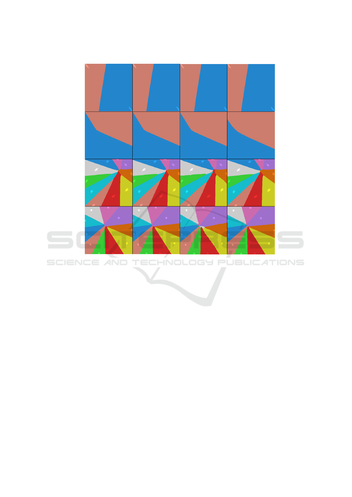
Logistic Regression SVM Random Forests Neural Network
10-class/700 dims 10-class/100 dims 2-class/700 dims 2-class/100 dims
Figure 2: Decision Boundary Maps (DBMs) created with SDBM for several classifiers (columns) and synthetic datasets (rows).
Lighter pixels represent training samples from the datasets D.
uses the full resolution of
G
to compute
P(D)
, but then
evaluates
P
−1
on a subsampled version thereof. In our
case, both
P
and
P
−1
use the full resolution image
G
.
For the experiments in this paper, we set the resolution
of G to 300
2
pixels.
4. Create Synthetic Data Points:
Use the trained
P
−1
to map each pixel
p ∈ G
2
to a high-dimensional
data point
x ∈ R
n
. This is similar to DBM, except the
use of a dense pixel grid and jointly-trained
P
and
P
−1
(see above).
5. Color Pixels:
Color all pixels
p ∈ G
by the values
of
f (P
−1
(p))
, i.e., the inferred classes of their corre-
sponding (synthetic) data points, using a categorical
color map. In this paper we use the ‘tab20’ color
map (Hunter, 2007). This is the same as DBM.
6. Encode Classifier Confidence (Optional):
For
classifiers
f
that provide the probability of a sample
x
belonging to a class
c
k
, we encode that probability
in the brightness of the pixel
p
that back-projects to
x
.
The lower the confidence of the classifier is, the darker
the pixel appears in the map, thereby informing the
user of the confidence of the decision zone in that area.
This is the same as DBM.
4 RESULTS
We next present the results that support our claims
regarding SDBM. First, we show how our method
performs with synthetic data, where a perfect class
separation is possible by most classifiers (Sec. 4.1).
This allows us to verify how the technique performs
under a controlled setting where we know the ‘ground
truth’ shapes of the decision zones. Next, we show how
SDBM performs on more complex real-world datasets
and additional classifiers (Sec. 4.2) and also how it
compares with DBM. This supports our claim that our
technique can be generically used and that it improves
quality vs DBM. We next show how SDBM compares
to the original DBM speed-wise, thereby supporting
our claims of improved scalability (Sec. 4.3). Finally,
we provide full implementation details for SDBM
(Sec. 4.4).
IVAPP 2022 - 13th International Conference on Information Visualization Theory and Applications
80
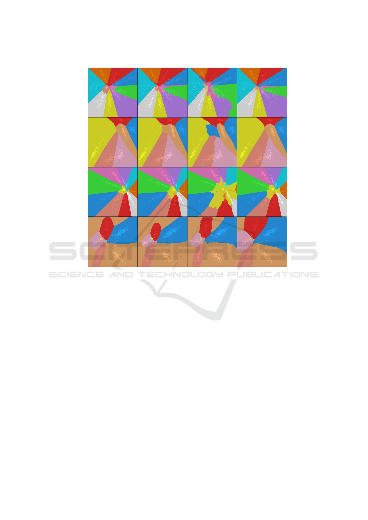
Logistic Regression SVM Random Forests Neural Network
Reuters MNIST HAR FashionMNIST
0.828 0.848 0.849 0.849
0.981 0.972 0.982 0.988
0.889 0.950 0.940 0.943
0.893 0.887 0.874 0.882
Figure 3: Decision Boundary Maps (DBMs) created with SDBM for several classifiers (columns) and real-world datasets
(rows). Numbers inside each map indicate test accuracy obtained by each classifier, bold indicating top performers. Lighter
pixels represent training samples from the datasets D.
4.1 Quality on Synthetic Datasets
We assess how SDBM performs in a controlled situ-
ation where the ground truth is known, i.e., datasets
with clear class separation and known shapes of the
expected decision zones. The datasets contain syn-
thetic Gaussian blobs with 5000 samples, with varied
dimensionality (100 and 700), and varied number of
classes (2 and 10). We used four different classifiers,
namely Logistic Regression, SVM (with a RBF ker-
nel), Random Forests (200 estimators), and a Neural
Network (multi-layer perceptron having 3 layers of
200 units).
Figure 2 shows the maps created using SDBM for
all the different classifier and dataset combinations.
Decision zones are categorically colored. Projected
samples in
P(D)
are drawn colored also by their class,
but slightly brighter, so as to distinguish them from
the maps. We see that the decision zones are com-
pact and with smooth boundaries, as expected for such
simple classification problems. They enclose the Gaus-
sian blobs with the same respective labels – e.g., the
red and blue zones for the 2-class, 100-dimensional
dataset in Fig. 2, top row, contain two clusters of light
red, respectively light blue, projected points. We also
see that the maps for Logistic Regression show almost
perfectly straight boundaries, which is a known fact for
this classifier. In contrast, the more sophisticated clas-
sifiers, such as Random Forests and Neural Networks,
create boundaries that are slightly more complex than
the others for the most complex dataset (Fig. 2, bottom
row, at the center of the maps for those classifiers).
4.2 Quality on Real-world Datasets
We next show how SDBM performs on real-world
datasets. These datasets are selected from publicly
available sources, matching the criteria of being high-
dimensional, reasonably large (thousands of samples),
and having a non-trivial data structure. They are also
frequently used in ML classification evaluations and
projection evaluations.
SDBM: Supervised Decision Boundary Maps for Machine Learning Classifiers
81
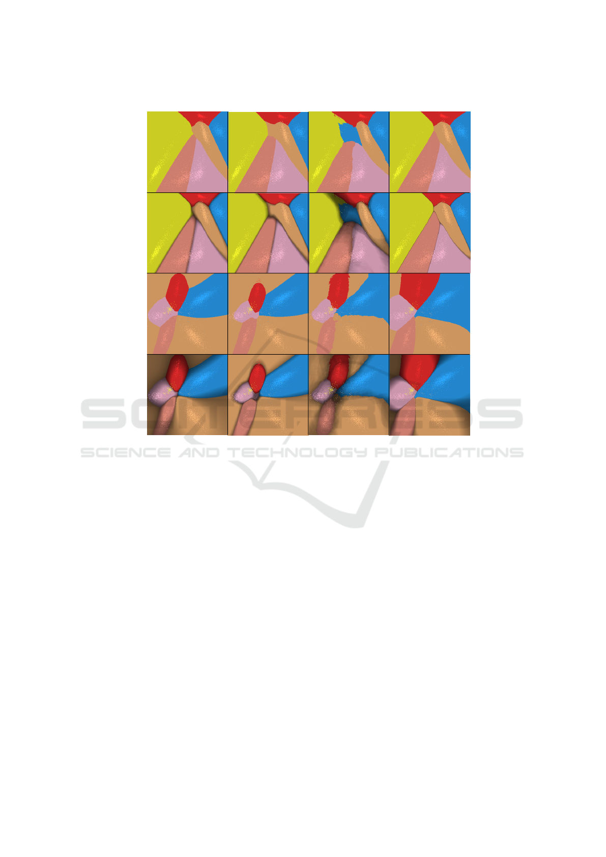
Logistic Regression SVM Random Forests Neural Network
Reuters (w/ conf) Reuters HAR (w/ conf) HAR
Figure 4: Decision Boundary Maps created with SDBM for several classifiers, HAR and Reuters datasets. Columns show
different classifiers. Rows show different datasets, with and without confidence encoded into brightness.
FashionMNIST
(Xiao et al., 2017)
:
70K samples of
K = 10
types of pieces of clothing, rendered as 28x28-
pixel gray scale images, flattened to 784-element vec-
tors. We also use a subset of this dataset containing
only two classes, namely Ankle Boot and T-Shirt, to
provide an example of a problem where classes are
more easily separable. This dataset was downsampled
to 10K observations for all uses in this paper.
Human Activity Recognition (HAR)
(Anguita et al.,
2012)
:
10299 samples from 30 subjects performing
K = 6
activities of daily living used for human activ-
ity recognition, described with 561 dimensions that
encode 3-axial linear acceleration and 3-axial angular
velocity measured on the subjects.
MNIST
(LeCun and Cortes, 2010)
:
70K samples
of
K = 10
handwritten digits from 0 to 9, rendered
as 28x28-pixel gray scale images, flattened to 784-
element vectors. This dataset was downsampled to
10K observations for all uses in this paper.
Reuters Newswire Dataset
(Thoma, 2017)
:
8432 ob-
servations of news report documents, from which 5000
attributes were extracted using TF-IDF (Salton and
McGill, 1986), a standard method in text processing.
This is a subset of the full dataset which contains data
for the K = 6 most frequent classes.
Figure 3 shows the maps created by SDBM for
these datasets, with the same types of classifiers used
in Sec. 4.1. Even though the current real-world
datasets are considerably more complex and harder
to separate into classes, the classifiers’ decision bound-
aries are clearly visible. Simpler classifiers (Logistic
Regression and SVM) show decision zones that are
more contiguous and have smoother, simpler, bound-
aries. More complex classifiers (Random Forests and
Neural Networks) show more complex shapes and
topologies of the decision zones. In particular, the
maps created for the Random Forest classifiers show
very jagged boundaries. This can be a result of having
an ensemble of classifiers working together.
Encoding Classifier Confidence:
Figure 4 shows
maps created by SDBM with classifier confidence en-
coded as brightness, as described in Sec. 3. This allows
us to see how different classifiers model probability
very differently, and thus produce different results.
IVAPP 2022 - 13th International Conference on Information Visualization Theory and Applications
82

The added value of encoding confidence can be seen
if we compare the first-vs-second, respectively third-
vs-fourth, rows in Fig. 4. The confidence-encoding
maps show a smooth brightness gradient, dark close
to the decision boundaries (where colors change in
the images) and bright deep in the decision zones.
The effect is slightly reminiscent of shaded cushion
maps (van Wijk and van de Wetering, 1999), i.e., it
enhances the visual separation of the color-coded de-
cision zones. More importantly, the shading gradi-
ent effectively shows how confidence increases as we
go deeper into the decision zones for different classi-
fiers: For example, for the HAR dataset, these shaded
bands are quite thin for Logistic Regression and SVM,
thicker and less informative for Random Forests, and
extremely and uniformly thin for Neural Networks.
This tells us that Neural Networks have an overall very
high confidence everywhere (except very close to the
decision boundaries); Logistic Regression and SVM
are less confident close to the boundaries; and Random
Forests have a higher variation of confidence over the
data space. For Random Forests, we see that the dark-
est region falls in the area of the central blue decision
zone and the top-right of the left yellow zone. This
are precisely the areas where the map of this classifier
significantly differs from those of all the other three
classifiers. Hence, we can infer that the isolated blue
decision zone that Random Forests created is likely
wrong, as it is low confidence and different from what
all the other three classifiers created in that area. For
the Reuters dataset (Fig. 4 bottom row), we see that
all classifiers produced a beige region at the top left
corner. The confidence information (brightness) shows
us that all classifiers but one (SVM) treat this region
as a low confidence one. This can be explained by the
total absence of training samples in that region. More
importantly, this tells us that the behavior of SVM in
this region is likely wrong.
Confidence visualization also serves in quickly and
globally assessing the overall quality of a trained clas-
sifier. Consider e.g. the Reuters dataset (Fig. 4 bot-
tom row). Compared to all other three rows in Fig. 4,
the decision maps for this dataset are darker. This
shows that this dataset is harder to extrapolate from
during inference. Note that this is not the same as the
usual testing-after-training in ML. Indeed, for testing,
one needs to ‘reserve’ a set of samples unseen dur-
ing training to evaluate the trained classifier on. In
contrast, SDBM’s decision maps do not need to do
this as they synthesize ‘testing’ samples on the fly via
the inverse projection
P
−1
. Moreover, classical ML
testing only gives a global or per-class accuracy. In
contrast, SDBM gives a per-region-of-the-data-space
confidence, encoded by brightness.
Comparison with the Original DBM:
Figure 5
shows maps created by SDBM side-by-side with maps
created by the original DBM technique, using Logistic
Regression, Random Forest and k-NN classifiers, for
three real-world datasets. In this experiment, we used
UMAP (McInnes and Healy, 2018) as the direct projec-
tion for DBM, and iLAMP (Amorim et al., 2012) for
the inverse projection, respectively Several important
observations can be made, as follows.
First, we see that the projections
P(D)
of the same
datasets are not the same with DBM and SDBM –
compare the bright-colored dots in the correspond-
ing figures. This is expected, since, as explained in
Sec. 3, DBM employs a user-chosen projection tech-
nique
P
, whereas SDBM learns
P
from the label-based
clustering of the data, following the SSNP method
(see Sec. 3). Since the projections
P(D)
of the same
datasets differ for the two methods, it is expected that
the overall shapes of the ensuing decision boundaries
will also differ – see e.g. the difference between the
nearly horizontal decision boundary between the blue
and red zones for Random Forests with DBM for Fash-
ionMNIST (2-class) and the angled boundary between
the same zones for the same classifier, same dataset,
with SDBM (Fig. 5, middle row, two leftmost images).
For the relatively simple classification problem that
FashionMNIST (2-class) is, this is not a problem. Both
DBM and SDBM produce useful and usable renditions
of the two resulting decision zones, showing that this
classification problem succeeded with no issues.
When considering more difficult datasets (Fashion-
MNIST 10-class or HAR), the situation is dramatically
different: DBM shows highly noisy pictures, where
it is even hard to say where and which are the actual
decision zones. These images suggest that none of
the three tested classifiers could correctly handle these
datasets, in the sense that they would change deci-
sions extremely rapidly and randomly as points only
slightly change over the data space. This is known not
to be the case for these datasets and classifiers. Logis-
tic Regression has built-in limitations of how quickly
its decision boundaries can change (Rodrigues et al.,
2019). k-NN is also known to construct essentially
a Voronoi diagram around the same-class samples in
the
n
D space, partitioning that space into cells whose
boundaries are smooth manifolds. DBM does not show
any such behavior (Fig. 5, third and fifth columns). In
contrast, SDBM shows a far lower noise level and
far smoother, contiguous, decision zones and bound-
aries. Even though we do not have formal ground
truth on how the zones and boundaries of these dataset-
classifier combinations actually look, SDBM matches
better the knowledge we have on these problems than
DBM.
SDBM: Supervised Decision Boundary Maps for Machine Learning Classifiers
83
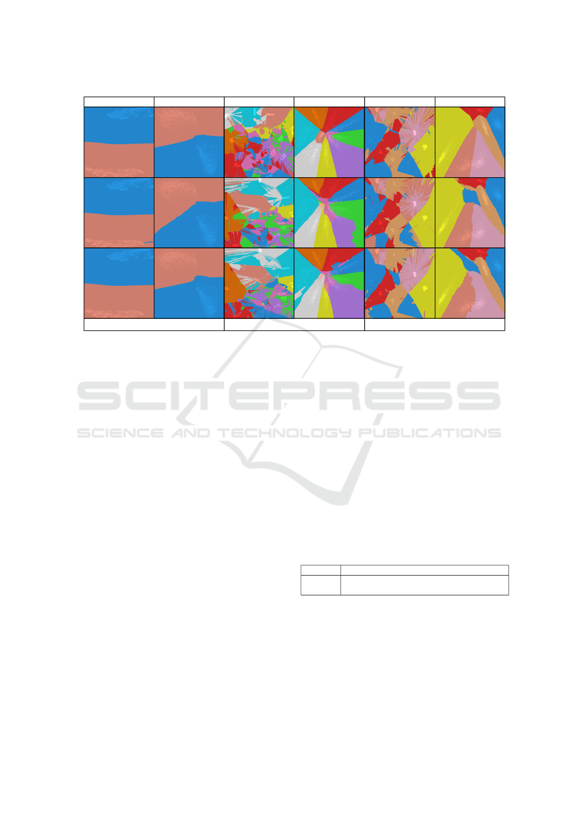
DBM SDBM
kNN Random Forests Logistic Regression
FashionMNIST (2-class) FashionMNIST (10-class) HAR
DBM SDBM
DBM SDBM
Figure 5: Comparison between SDBM and DBM using three different datasets and three classifiers.
4.3 Computational Scalability
We next study the scalability of SDBM and compare
it to the original DBM method. For this, we created
maps using synthetic Gaussian blobs datasets with 5
clusters, varying the dimensionality from 10 to 500,
and varying the map size from
25
2
to
300
2
pixels.
We did not use larger maps since the speed-trends
were already clear from these sizes, with DBM getting
considerably slower than SDBM. Figure 6 shows the
running times of both methods as a function of both the
grid size (horizontal axis) and dataset dimensionality
(different-color lines). We see that DBM’s runtime
increases quickly with dimensionality, taking about 5
minutes to create a
300
2
map for the 500-dimensional
dataset.
In contrast, SDBM is over an order of magni-
tude faster, taking roughly 7 seconds to run for the
same dataset. Also, we see that SDBM’s speed only
marginally depends on the dimensionality, whereas
this is a major slowdown factor for DBM. With re-
spect to the number of samples, we see that both meth-
ods exhibit similar trends, with SDBM being closer
to a linear trend than DBM. However, the slope of the
SDBM graphs is smaller than for DBM for the same
dimensionality. All in all, this shows that SDBM is
significantly more scalable than DBM. This can be ex-
plained by the fact that SSNP, which underlies SDBM,
jointly trains both the direct and inverse projections by
deep learning. As this is GPU-accelerated, linear in
the sample and dimension counts both for training and
inference, and does not need to use different resolu-
tions and sampling tricks for accelerating the 2D to
n
D
mapping (see Sec. 3). In contrast, DBM uses UMAP
and iLAMP for the direct, respectively, inverse projec-
tions (as mentioned earlier). None of these techniques
is GPU-accelerated.
4.4 Implementation Details
All experiments presented above were run on a dual 8-
core Intel Xeon Silver 4110 with 256 GB RAM and an
NVidia GeForce RTX 2070 GPU with 8 GB VRAM.
Table 1 lists all open-source software libraries used
to build SDBM and the other tested techniques. Our
implementation, plus all code used in this experiment,
are publicly available at (The Authors, 2021).
Table 1: Software packages used in the evaluation.
Technique Software used publicly available at
SSNP keras.io (TensorFlow backend) (Chollet and others, 2015)
UMAP github.com/lmcinnes/umap (McInnes and Healy, 2018)
5 DISCUSSION
We discuss how our technique performs with respect
to the criteria laid out in Section 1.
Quality (C1):
SDBM is able to create maps that show
classifier decision boundaries very clearly, and, most
importantly, much clearer than the maps created with
IVAPP 2022 - 13th International Conference on Information Visualization Theory and Applications
84
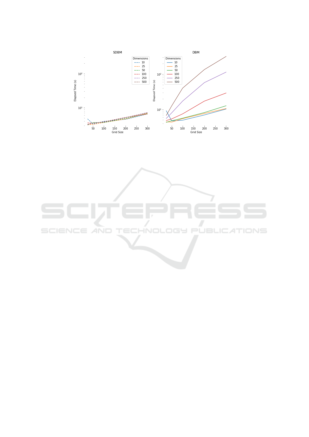
Figure 6: Plot showing the order of growth of time used to create maps of increasing size using DBM and SDBM, using
synthetic datasets of varying dimensionality. Vertical axis is in logarithmic scale.
the original DBM. For the same dataset-classifier com-
binations, SDBM’s maps show significantly less noise,
more compact decision zones, and smoother decision
boundaries, than DBM. These results are in line with
what we expect for dataset-classifier combinations for
which we have ground-truth knowledge about their
decision zones and boundaries (see Fig. 5 and related
text). As such, we conclude that SDBM captures the
actual decision zones better than DBM can do.
Scalability (C2):
SDBM is an order of magnitude
faster than DBM. Since SDBM scales linearly in the
number of observations during inference/drawing, and
it is end-to-end GPU-accelerated, it is able to generate
maps having hundreds of thousands of pixels in a few
seconds, which makes it practical for handling large
datasets and rendering highly detailed decision maps.
Ease of use (C3): SDBM produces good results with
minimal tuning. The single performance-sensitive set-
ting is the size of the map image. All maps in this paper
have
300
2
pixels. As the figures show, this resolution
is already sufficient for rendering detailed decision
maps for all the tested dataset-classifier combination.
Compared to DBM, SDBM tuning is far simpler, as
it does not require tuning of cell and sample sizes re-
quired by the former (for details of DBM tuning, we
refer to (Rodrigues et al., 2019)).
Genericity (C4):
As for the original DBM method,
SDBM is agnostic to the nature and dimensionality of
the input data, and to the classifier being visualized.
We show that SDBM achieves high quality on datasets
of different natures and coming from a wide range
of application domains, and with classifiers based on
quite different algorithms. As such, SDBM does not
trade any flexibility that DBM already offered, but
increases quality, scalability, and ease of use, as ex-
plained above.
Limitations:
SDBM shares a few limitations with
DBM. First and foremost, it is hard to formally assess
the quality of the decision maps it produces for dataset-
classifier combinations for which we do not have clear
ground-truth on the shape and position of their deci-
sion zones and boundaries. Current testing shown in
this paper has outlined that SDBM produces results
fully in line with known ground truth for such simple
situations. However, this does not formally guarantee
that the same is true for more complex datasets and
any classifiers. Finding ways to assess this is an open
problem to be studied in future work. Secondly, the
interpretation of the SDBM maps can be enhanced.
Examples shown in this paper outlined how such maps
can help finding out whether a trained classifier can
generalize well, and how far, from its training set, and
how different classifier-dataset combinations can be
compared by such maps. Yet, such evidence is qualita-
tive. A more formal study showing how users actually
interpret such maps to extract quantitative information
on the visualized classification problems is needed.
6 CONCLUSION
We have presented SDBM, a new method for produc-
ing classifier Decision Boundary Maps. Compared to
the only similar technique we are aware of – DBM –
our method presents several desirable characteristics.
First and foremost, it is able to create decision maps
which are far smoother and less noisy than those cre-
ated by DBM and also match the known ground-truth
of the visualized classification problems far better than
DBM, therefore allowing users to interpret the studied
classifiers with less confusion. Secondly, SDBM is
about an order of magnitude faster than DBM due to
its joint computation of direct and inverse projections
SDBM: Supervised Decision Boundary Maps for Machine Learning Classifiers
85

on a fixed-resolution image. Finally, SDBM has virtu-
ally no parameters to tune (apart from the resolution of
the desired final image) which makes it easier to use
than DBM.
Future work can target several directions. We be-
lieve a very relevant one to be the generation of maps
for multi-output classifiers, i.e., classifiers that can out-
put more than a single class for a sample. Secondly,
we consider organizing more quantitative studies to
actually gauge which are the interpretation errors that
SDBM maps generate when users consider them to
assess and/or compare the behavior of different clas-
sifiers, which is the core use-case that decision maps
have been proposed for. Thirdly, we consider adapting
SDBM to help the understanding of semantic segmen-
tation models. Last but not least, the packaging of
SDBM into a reusable library that can be integrated
into typical ML pipelines can help it gain widespread
usage.
ACKNOWLEDGMENTS
This study was financed in part by the Coordena
c¸
˜
ao
de Aperfei
c¸
oamento de Pessoal de N
´
ıvel Superior -
Brasil (CAPES) - Finance Code 001, and by FAPESP
grants 2015/22308-2, 2017/25835-9 and 2020/13275-
1, Brazil.
REFERENCES
Amorim, E., Brazil, E. V., Daniels, J., Joia, P., Nonato, L. G.,
and Sousa, M. C. (2012). iLAMP: Exploring high-
dimensional spacing through backward multidimen-
sional projection. In Proc. IEEE VAST, pages 53–62.
Anguita, D., Ghio, A., Oneto, L., Parra, X., and Reyes-Ortiz,
J. L. (2012). Human activity recognition on smart-
phones using a multiclass hardware-friendly support
vector machine. In Proc. Intl. Workshop on Ambient
Assisted Living, pages 216–223. Springer.
Breiman, L. (2001). Random forests. Machine learning,
45(1):5–32. Springer.
Chan, D., Rao, R., Huang, F., and Canny, J. (2018). T-SNE-
CUDA: GPU-accelerated t-SNE and its applications to
modern data. In Proc. SBAC-PAD, pages 330–338.
Chollet, F. and others (2015). Keras.
Cortes, C. and Vapnik, V. (1995). Support-vector networks.
Machine learning, 20(3):273–297. Springer.
Cox, D. R. (1958). The regression analysis of binary se-
quences. Journal of the Royal Statistical Society: Se-
ries B (Methodological), 20(2):215–232. Wiley Online
Library.
Cunningham, J. and Ghahramani, Z. (2015). Linear dimen-
sionality reduction: Survey, insights, and generaliza-
tions. JMLR, 16:2859–2900.
Engel, D., Hattenberger, L., and Hamann, B. (2012). A
survey of dimension reduction methods for high-
dimensional data analysis and visualization. In Proc.
IRTG Workshop, volume 27, pages 135–149. Schloss
Dagstuhl.
Espadoto, M., Hirata, N. S., and Telea, A. C. (2021). Self-
supervised dimensionality reduction with neural net-
works and pseudo-labeling. In Proc. IVAPP, pages
27–37. SCITEPRESS.
Espadoto, M., Hirata, N. S. T., and Telea, A. C. (2020). Deep
learning multidimensional projections. Information
Visualization, 19(3):247–269. SAGE.
Espadoto, M., Martins, R. M., Kerren, A., Hirata, N. S.,
and Telea, A. C. (2019a). Toward a quantitative sur-
vey of dimension reduction techniques. IEEE TVCG,
27(3):2153–2173.
Espadoto, M., Rodrigues, F. C. M., Hirata, N. S. T., Hi-
rata Jr., R., and Telea, A. C. (2019b). Deep learning
inverse multidimensional projections. In Proc. EuroVA.
Eurographics.
Garcia, R., Telea, A., da Silva, B., Torresen, J., and Comba,
J. (2018). A task-and-technique centered survey on
visual analytics for deep learning model engineering.
Computers and Graphics, 77:30–49. Elsevier.
Hoffman, P. and Grinstein, G. (2002). A survey of visualiza-
tions for high-dimensional data mining. Information
Visualization in Data Mining and Knowledge Discov-
ery, 104:47–82. Morgan Kaufmann.
Hunter, J. D. (2007). Matplotlib: A 2d graphics environ-
ment. Computing in science & engineering, 9(3):90–
95. IEEE.
Jolliffe, I. T. (1986). Principal component analysis and factor
analysis. In Principal Component Analysis, pages 115–
128. Springer.
LeCun, Y. and Cortes, C. (2010). MNIST handwritten digits
dataset. http://yann.lecun.com/exdb/mnist.
Liu, S., Maljovec, D., Wang, B., Bremer, P.-T., and Pas-
cucci, V. (2015). Visualizing high-dimensional data:
Advances in the past decade. IEEE TVCG, 23(3):1249–
1268.
Lundberg, S. M. and Lee, S.-I. (2017). A unified approach
to interpreting model predictions. In Proc. NIPS, pages
4768–4777.
Maaten, L. v. d. (2014). Accelerating t-SNE using tree-based
algorithms. JMLR, 15:3221–3245.
Maaten, L. v. d. and Hinton, G. (2008). Visualizing data
using t-SNE. JMLR, 9:2579–2605.
Maaten, L. v. d. and Postma, E. (2009). Dimensionality
reduction: A comparative review. Technical report,
Tilburg University, Netherlands.
McInnes, L. and Healy, J. (2018). UMAP: Uniform manifold
approximation and projection for dimension reduction.
arXiv:1802.03426v1 [stat.ML].
Nonato, L. and Aupetit, M. (2018). Multidimensional pro-
jection for visual analytics: Linking techniques with
distortions, tasks, and layout enrichment. IEEE TVCG.
Pezzotti, N., H
¨
ollt, T., Lelieveldt, B., Eisemann, E., and
Vilanova, A. (2016). Hierarchical stochastic neighbor
embedding. Computer Graphics Forum, 35(3):21–30.
Wiley Online Library.
IVAPP 2022 - 13th International Conference on Information Visualization Theory and Applications
86

Pezzotti, N., Lelieveldt, B., Maaten, L. v. d., H
¨
ollt, T., Eise-
mann, E., and Vilanova, A. (2017). Approximated and
user steerable t-SNE for progressive visual analytics.
IEEE TVCG, 23:1739–1752.
Pezzotti, N., Thijssen, J., Mordvintsev, A., Hollt, T., Lew,
B. v., Lelieveldt, B., Eisemann, E., and Vilanova, A.
(2020). GPGPU linear complexity t-SNE optimization.
IEEE TVCG, 26(1):1172–1181.
Rauber, P. E., Fadel, S. G., Falcao, A. X., and Telea, A. C.
(2017a). Visualizing the hidden activity of artificial
neural networks. IEEE TVCG, 23(1):101–110.
Rauber, P. E., Falcao, A. X., and Telea, A. C. (2017b). Pro-
jections as visual aids for classification system design.
Information Visualization, 17(4):282–305. SAGE.
Ribeiro, M. T., Singh, S., and Guestrin, C. (2016). Why
should i trust you?: Explaining the predictions of any
classifier. In Proc. ACM SIGMOD KDD, pages 1135–
1144.
Rodrigues, F., Espadoto, M., Hirata, R., and Telea, A. C.
(2019). Constructing and visualizing high-quality clas-
sifier decision boundary maps. Information, 10(9):280.
MDPI.
Roweis, S. T. and Saul, L. L. K. (2000). Nonlinear di-
mensionality reduction by locally linear embedding.
Science, 290(5500):2323–2326. AAAS.
Salton, G. and McGill, M. J. (1986). Introduction to modern
information retrieval. McGraw-Hill.
Sorzano, C., Vargas, J., and Pascual-Montano, A. (2014).
A survey of dimensionality reduction techniques.
arXiv:1403.2877 [stat.ML].
Tenenbaum, J. B., Silva, V. D., and Langford, J. C. (2000).
A global geometric framework for nonlinear dimen-
sionality reduction. Science, 290(5500):2319–2323.
AAAS.
The Authors (2021). SDBM implementation. https://github.
com/mespadoto/sdbm.
Thoma, M. (2017). The Reuters dataset. https://
martin-thoma.com/nlp-reuters.
Torgerson, W. S. (1958). Theory and Methods of Scaling.
Wiley.
van Wijk, J. J. and van de Wetering, H. (1999). Cushion
treemaps: Visualization of hierarchical information. In
Proc. InfoVis.
Wattenberg, M. (2016). How to use t-SNE effectively. https:
//distill.pub/2016/misread-tsne.
Xiao, H., Rasul, K., and Vollgraf, R. (2017). Fashion-
MNIST: A novel image dataset for benchmarking ma-
chine learning algorithms. arXiv:1708.07747.
Xie, H., Li, J., and Xue, H. (2017). A survey of dimension-
ality reduction techniques based on random projection.
arXiv:1706.04371 [cs.LG].
SDBM: Supervised Decision Boundary Maps for Machine Learning Classifiers
87
