Adversarial Examples by Perturbing High-level Features in Intermediate
Decoder Layers
Vojt
ˇ
ech
ˇ
Cerm
´
ak and Luk
´
a
ˇ
s Adam
a
Faculty of Electrical Engineering, Czech Technical University in Prague, Technick
´
a 2, Prague, Czech Republic
Keywords:
Adversarial Examples, Robust Machine Learning, Representation Learning, High-level Features,
Intermediate Latent Representation.
Abstract:
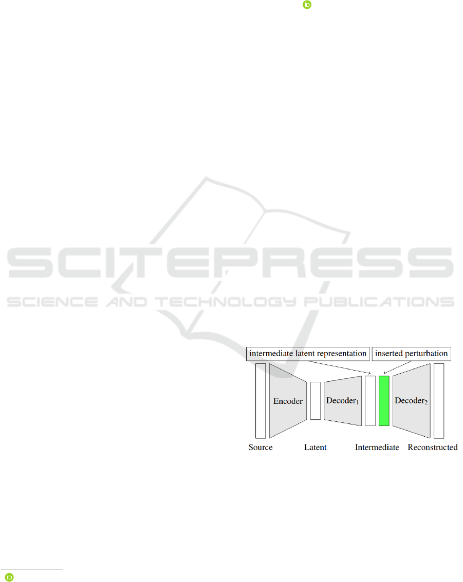
We propose a novel method for creating adversarial examples. Instead of perturbing pixels, we use an encoder-
decoder representation of the input image and perturb intermediate layers in the decoder. This changes the
high-level features provided by the generative model. Therefore, our perturbation possesses semantic meaning,
such as a longer beak or green tints. We formulate this task as an optimization problem by minimizing
the Wasserstein distance between the adversarial and initial images under a misclassification constraint. We
employ the projected gradient method with a simple inexact projection. Due to the projection, all iterations are
feasible, and our method always generates adversarial images. We perform numerical experiments by fooling
MNIST and ImageNet classifiers in both targeted and untargeted settings. We demonstrate that our adversarial
images are much less vulnerable to steganographic defence techniques than pixel-based attacks. Moreover, we
show that our method modifies key features such as edges and that defence techniques based on adversarial
training are vulnerable to our attacks.
1 INTRODUCTION
In the past decade, the widespread application of deep
neural networks raised security concerns as it creates
incentives for attackers to exploit any potential weak-
ness. For example, attackers could create traffic signs
invisible to autonomous cars or make malware filters
ignore threats. Those security concerns rose since
(Szegedy et al., 2014) showed that deep neural net-
works are vulnerable to small perturbations of inputs
that are designed to cause misclassification of a classi-
fier. These adversarial examples are indistinguishable
from natural examples as the perturbation is too small
to be perceived by humans.
We extend the usual approach to constructing
adversarial examples that focuses on norm-bounded
pixel modifications. Instead of perturbing the pixels
directly, we perturb features learned by an encoder-
decoder model. There are several ways to perturb
the features from the decoder, ranging from high-level
features collected from initial decoder layers to much
finer features collected from decoder layers near the
reconstructed image. When we perturb features in
the initial layers near the latent image representation,
a
https://orcid.org/0000-0001-8748-4308
even small perturbations may completely change the
image meaning. On the other hand, perturbations on
fine features are very close to pixel perturbations and
carry little semantic information. As a compromise,
we suggest perturbing intermediate decoder layers.
Figure 1.
Our way of generating adversarial images pro-
vides several advantages:
• The perturbations are interpretable. They mod-
ify high-level features such as fur colour or beak
length.
• The perturbations often follow edges. This means
that they are less detectable by steganographic de-
fence techniques (Johnson and Jajodia, 1998).
496
ˇ
Cermák, V. and Adam, L.
Adversarial Examples by Perturbing High-level Features in Intermediate Decoder Layers.
DOI: 10.5220/0010892800003116
In Proceedings of the 14th International Conference on Agents and Artificial Intelligence (ICAART 2022) - Volume 2, pages 496-507
ISBN: 978-989-758-547-0; ISSN: 2184-433X
Copyright
c
 2022 by SCITEPRESS – Science and Technology Publications, Lda. All rights reserved

• The perturbations keep the structure of the unper-
turbed images, including hidden structures unre-
lated to their semantic meaning.
• The decoder ensures that the adversarial images
have the correct pixel values; there is no need to
project to [0,1].
The drawback of our approach is that we cannot per-
turb an arbitrary image but only those representable
by the decoder.
To obtain a formal optimization problem, we min-
imize the distance between the original and adversar-
ial images in the reconstructed space. To successfully
generate an adversarial image, we add a constraint re-
quiring that the perturbed image is misclassified. To
handle this constraint numerically, we propose to use
the projected gradient method. We approximate the
projection operator by a fast method which always re-
turns a feasible point. This brings additional benefits
to our method:
• The method works with feasible points. Even if it
does not converge, it produces an adversarial im-
age.
• Because we minimize the distance between the
original and adversarial images, we do not need to
specify their maximal possible distance as many
methods do.
Numerical experiments present results on samples
from MNIST and ImageNet in both targeted and un-
targeted settings. They support all advantages men-
tioned above. We use both the l
2
and Wasserstein dis-
tances and show in which settings each performs bet-
ter. We select a simple steganography defence mech-
anism and show that our attack is much less vulnera-
ble to it than pixel-based perturbations. We examine
the difference between perturbing the latent and in-
termediate layers and show that the intermediate lay-
ers indeed modify the high-level features of the re-
constructed image. Finally, we show how our algo-
rithm gradually incorporates the high-level features
from the initial to the adversarial image. Our codes
are available online to promote reproducibility.
1
1.1 Related Work
The threat model based on small l
p
norm-bounded
perturbations has been the main focus of research. It
was originally introduced in (Szegedy et al., 2014),
where they used L-BFGS to minimize the l
2
distance
between the original and adversarial images. Since
then, many new ways how to both attack and defend
against adversarial examples have been introduced.
1
https://github.com/VojtechCermak/latent-adv-examples
(Goodfellow et al., 2015) introduced Fast Gradient
Sign Method (FGSM), which is bounded by the l
∞
metric. The authors used FGSM to generate new
adversarial examples and used them to augment the
training set in the adversarial training defence tech-
nique. A natural way to extend the FGSM attack is to
iterate the gradient step as it is done in the Basic Iter-
ative Method of (Kurakin et al., 2016) and Projected
Gradient Descend attack of (Madry et al., 2018). (Pa-
pernot et al., 2016) argued to use the l
0
distance to
model human perception and proposed a class of at-
tacks optimized under l
0
distance. (Carlini and Wag-
ner, 2017) designed strong attack algorithms based on
optimizing the l
0
, l
2
and l
∞
distances.
(Xiao et al., 2018) used GANs to generate noise
for adversarial perturbation. Other authors used gen-
erative models in defence against adversarial exam-
ples. MagNet of (Meng and Chen, 2017) used recon-
struction error of variational autoencoders to detect
adversarial examples. A similar idea was used in De-
fenceGAN of (Samangouei et al., 2018), where they
cleaned adversarial images by matching them to their
representation in latent space of the GAN trained on
clean data.
We use similar optimization techniques as in
decision-based attacks such as Boundary attack of
(Brendel et al., 2018) and HopSkipJump attack of
(Chen et al., 2020). The optimization techniques al-
ways keep intermediate results in the adversarial re-
gion and always outputs misclassified examples.
Some works have already investigated adversarial
examples outside of the l
p
norm. (Wong et al., 2019)
used the Sinkhorn approximation of the Wasserstein
distance to create adversarial images with the same
geometrical structure as the original images. The
Wasserstein distance is based on the cost needed
to move mass between two probability distributions.
Compared to standard distance metrics, such as l
2
dis-
tance, it includes information about the spatial distri-
bution of pixels. This makes the Wasserstein distance
more suitable for adversarial examples than the stan-
dard l
p
distance metrics because it can capture differ-
ences in high-level features. We increase this benefit
by additionally modifying the high-level features in-
stead of pixels.
The Unrestricted Adversarial Examples of (Song
et al., 2018), are adversarial examples constructed
from scratch using conditional generative models.
Our paper differs in several aspects. First, we use
the intermediate instead of the latent representation
to perturb high-level features. Second, we use an un-
conditional generator, which allows us to freely move
in the intermediate latent space and perform several
operations such as the projection.
Adversarial Examples by Perturbing High-level Features in Intermediate Decoder Layers
497

2 PROPOSED FORMULATION
Finding an adversarial image amounts to finding some
image x which is close to a given x
0
, and the neu-
ral network misclassifies it. For reasons mentioned in
the introduction, we do not work with the original im-
ages but with their latent representations. Therefore,
we need a decoder D which maps the latent repre-
sentation z to the original representation x. Since we
want to insert some perturbation p to the intermedi-
ate layer in the decoder, we split the decoder into two
parts D = D
2
◦ D
1
. We call D
1
(z) the intermediate
latent representation and D
2
(D
1
(z)) the reconstructed
image.
The mathematical formulation of finding an ad-
versarial image close to x
0
reads:
minimize
p
distance(x,x
0
)
subject to x = D
2
(D
1
(z
0
) + p),
x
0
= D
2
(D
1
(z
0
)),
g(x) ≤ 0,
x ∈ [0,1]
n
.
(1)
Here, z
0
is the latent representation of the image x
0
.
We insert the perturbation p to the intermediate latent
representation D
1
(z
0
) and only then reconstruct the
image by applying the second part of the decoder D
2
.
When D
1
is the identity, and D
2
is the decoder, we
obtain the case when perturbations appear in the la-
tent space. Similarly, when D
1
is the decoder, and D
2
is the identity, we recover the standard pixel perturba-
tions. Therefore, our formulation (1) generalizes both
approaches.
2.1 Objective
The objective function measures the distance between
the adversarial x and the original x
0
image in the re-
constructed space. We will use the l
2
norm and the
Wasserstein distance. Having the distance in the ob-
jective is advantageous because we do not need to
specify the ε-neighborhood when this distance is in
the constraint.
2.2 Constraints
Formulation (1) has multiple constraints. Constraint
x ∈ [0,1]
n
says that the pixels need to stay in this
range. Since x is an output of the decoder, this con-
straint is always satisfied.
The other constraint g(x) ≤ 0 is a misclassification
constraint. We employ the margin function
m(x,k) = max
i,i6=k
F
i
(x) −F
k
(x), (2)
where F = [F
1
(x),...,F
m
(x)] is a classifier with m
classes and k is a class index. We define this con-
straint for both targeted and untargeted attacks:
targeted : g(x) = m(x, k),
untargeted : g(x) = −m(x, argmax
i=1,...,m
F
i
(x)).
(3)
For the targeted case, we need to specify the target
class k, while for the untargeted case, the class k is
the classifier prediction. For the latter case, we need
to multiply the margin by −1 as we require the mis-
classified images to satisfy g(x) ≤ 0.
We will later use that the original image always
satisfies g(x
0
) > 0 because otherwise the original im-
age is already misclassified, and no perturbation (p =
0) is the optimal solution of (1).
3 PROPOSED SOLUTION
METHOD
We propose to solve (1) by the projected gradient
method (Nocedal and Wright, 2006) with inexact pro-
jection. Our algorithm produces a feasible point at
every iteration. Therefore, it always generates a mis-
classified image.
3.1 Proposed Algorithm
Since we optimize with respect to p, we define the
objective and constraint by
f (p) = distance(D
2
(D
1
(z
0
) + p),x
0
),
ˆg(p) = g(D
2
(D
1
(z
0
) + p)).
(4)
We describe our procedure in Algorithm 1. First, we
initialize p by some feasible p
init
and then run the
projected gradient method for max
iter
iterations. Step
8 computes the optimization step by minimizing the
objective f and step 9 uses the inexact projection (de-
scribed later) to project the suggested iteration p
next
back to the feasible set. As we will see later, the
constraint p
next
6= p implies that p
next
was not feasi-
ble, and it was projected onto the boundary. In such
a case, steps 4-7 “bounce away” from the boundary.
Since −∇ ˆg(p) points inside the feasible set, step 5
finds some β > 0 such that p − β∇ ˆg(p) lies in the in-
terior of the feasible set.
3.2 Inexact Projection
Step 9 in Algorithm 1 uses the inexact projection.
We summarize this projection in Algorithm 2. Its
main idea is to find a feasible point on the line be-
tween p and p
next
. This line is parameterized by
ICAART 2022 - 14th International Conference on Agents and Artificial Intelligence
498

Algorithm 1: For finding adversarial images by solving (1).
1: p ← p
init
2: for i ∈ {0,...,max
iter
} do
3: if i > 0 and p
next
6= p then
4: β ← β
i
5: while ˆg(p − β∇ ˆg(p)) ≥ 0 do
6: β ←
β
2
7: p ← p − β∇ ˆg(p)
8: p
next
← p −α
i
∇ f (p)
9: p ← PROJECT(p
next
, p,δ)
10: return p
(1 − c)p + cp
next
for c ∈ [0,1]. Due to the construc-
tion of Algorithm 1, p is always strictly feasible and
therefore ˆg(p) < 0. If ˆg(p
next
) < 0, then p
next
is fea-
sible and we accept it in step 4. In the opposite case,
we have ˆg(p) < 0 and ˆg(p
next
) ≥ 0 and we can use the
bisection method to find some c ∈ (0,1) for which the
constraint is satisfied. The standard bisection method
would return a point with ˆg((1 − c)p + cp
next
) = 0,
however, since the formulation (1) contains the in-
equality constraint, we require the constraint value to
lie only in some interval [−δ,0] instead of being zero.
Algorithm 2: Inexact projection onto the feasible set.
1: procedure PROJECT(p
next
, p,δ)
2: assert ˆg(p) < 0
3: if ˆg(p
next
) < 0 then
4: return p
next
5: a ← 0, b ← 1, c ←
1
2
(a +b)
6: while ˆg((1 − c)p +cp
next
) /∈ [−δ,0] do
7: if ˆg((1 −c)p +cp
next
) > 0 then
8: b ← c
9: else
10: a ← c
11: c ←
1
2
(a +b)
12: return (1 − c)p + cp
next
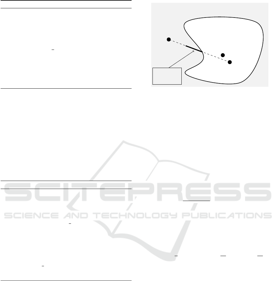
Figure 2 depicts the projection in the intermediate
latent space. The light-grey region is feasible, and
the white region is infeasible. The infeasible region
always contains D
1
(z
0
), while the feasible region al-
ways contains D
1
(z
0
) + p. If D
1
(z
0
) + p
next
lies in
the feasible region, the projection returns p
next
. In
the opposite case, we look for some point on the line
between D
1
(z
0
) + p and D
1
(z
0
) + p
next
. The points
which may be accepted are depicted by the thick solid
line. The length of this line is governed by the thresh-
old δ. The extremal case δ = 0 always returns the
point on the boundary, while δ = ∞ prolongs the line
to D
1
(z
0
) + p.
Feasible region
Infeasible region
D
1
(z
0
) + p
next
D
1
(z
0
) + p
D
1
(z
0
)
Accepted
projection
Figure 2: Inexact projection in the intermediate latent space.
The points which may be accepted are depicted by the thick
solid line.
3.3 Analysis of the Algorithm
The preceding text mentioned that Algorithm 1 gen-
erates a strictly feasible point p, thus g(D
2
(D
1
(z
0
) +
p)) < 0. We prove this in the next theorem and add a
speed of convergence.
Theorem 1. Assume that g◦ D
2
is a continuous func-
tion. Then Algorithm 2 generates a strictly feasible
point in a finite number of iterations. If g◦D
2
is more-
over Lipschitz continuous with modulus L, then Algo-
rithm 2 either immediately returns p
next
or converges
in at most log
2
Lkp
next
−pk
min{δ,− ˆg(p)}
iterations.
Proof. If ˆg(p
next
) < 0, then the algorithm immedi-
ately terminates. Assume thus ˆg(p
next
) ≥ 0. Denote
the iterations from Algorithm 2 by b
k
and a
k
with the
initialization b
0
= 1 and a
0
= 0. Since the interval
halves at each iteration, we obtain
b
k
− a
k
=
1
2
(b
k−1
− a
k−1
) =
1
2
k
(b
0
− a
0
) =
1
2
k
. (5)
Define
˜g(c) = ˆg((1 − c)p + cp
next
).
Since we have
˜g(b
0
) = ˜g(1) = ˆg(p
next
) ≥ 0,
˜g(a
0
) = ˜g(0) = ˆg(p) < 0.
due to the construction of the algorithm, we have
˜g(b
k
) ≥ 0 and ˜g(a
k
) < 0 for all k. Since ˜g is a contin-
uous function due to continuity of D
2
◦ g, Algorithm
2 converges in a finite number of iterations.
Assume that g ◦D
2
is a Lipschitz continuous func-
tion with modulus L, then ˆg is also Lipschitz continu-
Adversarial Examples by Perturbing High-level Features in Intermediate Decoder Layers
499

ous with modulus L. Then
| ˜g(c
1
) − ˜g(c
2
)|
= | ˆg((1 − c
1
)p + c
1
p
next
) − ˆg((1 − c
2
)p + c
2
p
next
)|
≤ Lk(1 − c
1
)p + c
1
p
next
− (1 − c
2
)p − c
2
p
next
k
= Lk(p
next
− p)(c
1
− c
2
)k
≤ Lkp
next
− pk|c
1
− c
2
|
Therefore, ˜g is a Lipschitz continuous function with
constant Lkp
next
− pk. Together with (5) this implies
˜g(b
k
) − ˜g(a
k
) ≤ Lkp
next
− pk(b
k
− a
k
)
= Lkp
next
− pk
1
2
k
.
(6)
If the algorithm did not finish within k itera-
tions, there are two possibilities. The first possibility
˜g(a
0
) < −δ implies ˜g(a
k
) < −δ. The second possi-
bility ˜g(a
0
) ∈ [−δ,0] implies ˜g(a
k
) ≤ ˜g(a
0
) because
otherwise the algorithm would have stopped already.
Both possibilities imply
˜g(b
k
) − ˜g(a
k
) ≥ − ˜g(a
k
) ≥ min{δ, − ˆg(p)}. (7)
The comparison of (6) and (7) implies that the algo-
rithm cannot run for more than the number of itera-
tions specified in the theorem statement.
The previous theorem implies that all iterations p
produced by Algorithm 1 are strictly feasible. The
theorem also provides another explanation why Algo-
rithm 1 must bounce away from the boundary in steps
4-7. If these steps were not present, ˆg(p) would of-
ten converge to zero and the number of iterations for
Algorithm 2 would increase to infinity.
4 EXPERIMENTAL SETUP
This section describes the experimental setup.
4.1 Used Architectures
As the classifiers to be fooled in our MNIST experi-
ments, we train a non-robust classifier with architec-
ture based on VGG blocks (Simonyan and Zisserman,
2015) and use the approach of (Madry et al., 2018)
to train robust networks with respect to l
2
and l
∞
at-
tacks. We generate new digits using an unconditional
ALI generator (Donahue et al., 2016; Dumoulin et al.,
2016). For ImageNet we use EfficientNet B0 (Tan and
Le, 2019) as a classifier and BigBiGAN (Donahue
and Simonyan, 2019) as an encoder-decoder model.
4.2 Numerical Setting
As an objective we use the standard l
2
distance and the
Sinkhorn approximation (Cuturi, 2013) to the Wasser-
stein distance. This approximation adds a weighted
Kullback-Leibler divergence to solve
minimize
W
hC,W i + λhW,logW i
subject to W 1 = x
0
,W
>
1 = x,W ≥ 0.
(8)
The optimal value of this problem is the Sinkhorn dis-
tance between images x
0
and x. The matrix C speci-
fies the distance between pixels. Since x
0
and x are
required to be probability distributions, we normal-
ize the pixels from decoder output to sum to one.
We do not need to impose the non-negativity con-
straint because the decoder outputs positive pixel in-
tensities. We use the implementation from the Geom-
Loss package (Feydy et al., 2019). Since the number
of elements W from (8) equals the number of pixels
squared, using the Sinkhorn distance was infeasible
for ImageNet, where we use only the l
2
distance.
For MNIST experiments, we randomly generate
the latent images z
0
and then use the decoder for re-
constructed images x
0
. We required that the classi-
fier predicts the digit into the correct class with the
probability of at least 0.99. For ImageNet, this tech-
nique produces images of lower quality, and we fed
the encoder with real images and used their encoded
representation.
We run all experiments for 1000 iterations. Algo-
rithm 1 requires stepsizes α and β, while Algorithm
2 requires the threshold δ. We found that the stepsize
α is not crucial because even if it is large, the projec-
tion will reduce it. We therefore selected α = 1. For
the second stepsize β, we selected a simple anneal-
ing scheme with exponential decay. In both cases, we
used the normed gradient. For the threshold we se-
lected δ = 1. Since the margin function (2) is bounded
by 1, Figure 2 then implies that the acceptable projec-
tion increases all the way to D
1
(z
0
)+ p. Since at least
one iteration of the projection is performed, the dis-
tance to the boundary at least halves. We found this
to be a good compromise between speed and approx-
imative quality. Theorem 1 then implies that Algo-
rithm 1 converges in at most log
2
L iterations.
We run our experiments on an Nvidia GPU with
6GB of VRAM.
4.3 Evaluation Metrics
Besides standard evaluation metrics, we also use
the least significant bit metric, which is a standard
steganographic defence technique to capture changes
ICAART 2022 - 14th International Conference on Agents and Artificial Intelligence
500

in the hidden structure of the data. For pixel intensi-
ties in x ∈ [0,1], it is defined by
lsb(x) = mod(round(255x), 2). (9)
Therefore, it transforms the image x ∈ [0,1] into its 8-
bit representation and takes the last (least significant)
bit.
5 EXPERIMENT RESULTS
This section presents numerical experiments to sup-
port our key claims from the introduction. Here, we
only present a short summary of both qualitative and
quantitative results. We postpone thorough descrip-
tions of our results to the next sections.
Qualitative results:
• Figures 4 and 5 show that our algorithm pro-
duces interpretable adversarial examples that fol-
low edges and does not break the structure of the
original dataset.
• Figure 7 shows how the choice of intermediate
layer affects the interpretation of perturbations
created by our algorithm.
• Figure 6 documents how the interpretability of our
perturbations naturally emerges due to the con-
struction of our algorithm.
Quantitative results :
• Table 1 shows that our algorithm often produces
reasonably strong attacks against both standard
and robust networks.
• Table 2 shows that our algorithm keeps the hidden
structure of the original data better than the CW
attack.
We split the discussion for results on the image
datasets MNIST (LeCun et al., 2010) and ImageNet
(Deng et al., 2009).
5.1 Numerical Results for MNIST
For the numerical experiments, we use the notation
of l
2
and Wasserstein attacks based on the objective
function in the model (1). For MNIST, we would like
to stress that none of the images was manually se-
lected, and all images were generated randomly.
Figure 3 shows targeted l
2
attacks (left) and tar-
geted Wasserstein attacks (right). Even though both
attacks performed well, the Wasserstein attack shows
fewer grey artefacts around the digits. This is natu-
ral as the Wasserstein distance considers the spatial
distribution of pixels. The is not the case for the l
2
distance.
Tables 1 and 2 show a numerical comparison be-
tween these two attacks and the CW l
2
attack (Car-
lini and Wagner, 2017) implemented in the Foolbox
library (Rauber et al., 2020). Besides the targeted at-
tacks, we also implemented untargeted attacks and at-
tacks against robust networks (additional figures are
in the appendix). The two robust networks were
trained to be robust with respect to l
2
and l
∞
attacks.
Table 1 shows the l
2
and Wasserstein distances.
The table shows that if we optimize with respect to
the Wasserstein distance, the Wasserstein distance be-
tween the original and adversarial images (column 8)
is the smallest. The same holds for the l
2
distance
(column 4). Even though the CW attack generated
smaller values in the l
2
distance, this happened be-
cause it is not restricted by the decoder. Moreover, as
we will see from the next figure, the CW attack gener-
ates lower-quality images which do not keep the hid-
den structure of the original images. It is also not sur-
prising that the needed perturbations are smaller for
untargeted attacks and the non-robust network. This
table demonstrates that our attacks are better in met-
rics that capture high-level features (Wasserstein dis-
tance).
Table 2 shows that our attack keeps the hidden
structure intact when compared to standard pixel-
based attacks. The right part shows the average frac-
tion of modified pixels, while the left side shows the
average fraction of modified least significant bits (9)
between the original and perturbed images. The table
shows that our algorithm is superior in both metrics.
Moreover, compared to standard pixel-based attacks,
our attacks yields consistent results in those metric
even when evaluated on robust models.
Figure 4 shows a visual comparison for untargeted
attacks. It shows the original image (left) and the CW
(middle left), l
2
(middle right) and Wasserstein (right)
attacks. Each three columns contain the adversarial
image, the least significant bit representation (9) and
the difference between the original and adversarial
images. A significant difference between our attacks
and the pixel-based CW attack is that our attacks pro-
vide interpretability of perturbations. Figure 4 shows
that there is no clear pattern in the pixel perturba-
tions of the CW attack, neither in the least significant
bit nor in the (almost) uniformly distributed perturba-
tions. On the other hand, our method keeps the least
significant bit structure. This implies that the least
significant bit defence can easily recognize the CW
attack, while our attacks cannot be recognized. At the
same time, our methods concentrate the attack around
the edges of the image. Therefore, our attacks are
compatible with the basic steganographic rule stating
that attacks should be concentrated mainly around key
Adversarial Examples by Perturbing High-level Features in Intermediate Decoder Layers
501

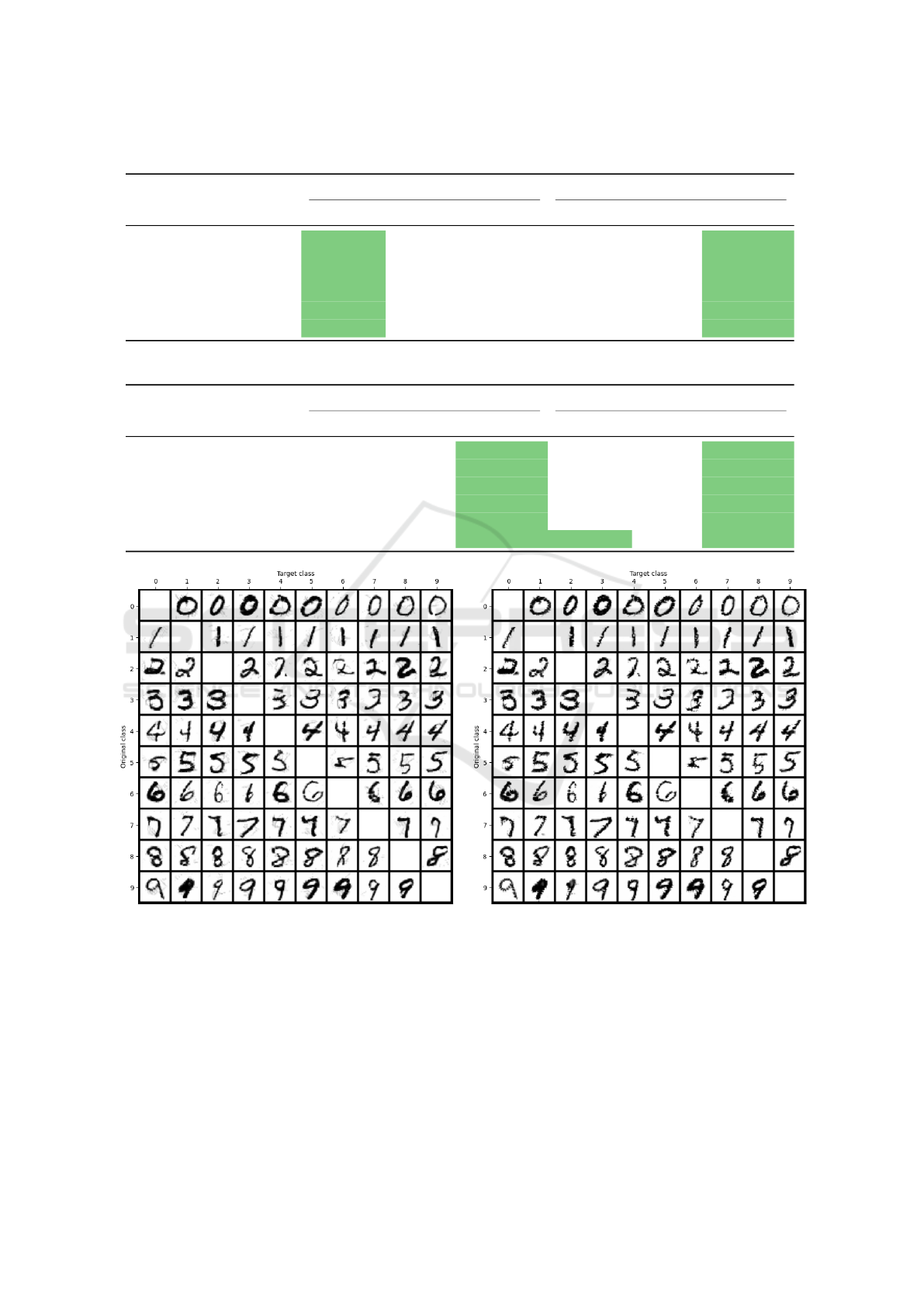
Table 1: Mean l
2
and Wasserstein distances between original and adversarial images over 90 randomly selected images.
Network Attack l
2
distance Wasserstein distance
CW attack l
2
attack Wasserstein CW attack l
2
attack Wasserstein
Non-robust Targeted 10.07 16.78 24.01 2.76 1.83 0.12
Untargeted 7.85 15.28 20.87 1.77 1.49 0.08
Robust l
2
Targeted 28.33 33.56 47.88 3.47 5.60 1.08
Untargeted 22.50 29.06 42.34 2.42 4.20 0.80
Robust l
in f
Targeted 23.51 29.56 35.63 1.11 3.84 0.46
Untargeted 19.26 25.44 31.04 0.58 2.53 0.31
Table 2: Metrics of change in structure between original and adversarial images over 90 randomly selected images.
Network Attack Fraction of modified LSB Fraction of modified pixels
CW attack l
2
attack Wasserstein CW attack l
2
attack Wasserstein
Non-robust Targeted 0.33 0.20 0.15 0.58 0.33 0.25
Untargeted 0.32 0.19 0.14 0.55 0.32 0.24
Robust l
2
Targeted 0.26 0.18 0.16 0.40 0.30 0.27
Untargeted 0.22 0.18 0.16 0.34 0.29 0.27
Robust l
in f
Targeted 0.17 0.17 0.15 0.28 0.29 0.26
Untargeted 0.16 0.17 0.15 0.25 0.28 0.25
Figure 3: Targeted l
2
attacks (left) and Wasserstein attacks (right). Rows represent the original while columns the target class.
features such as edges. We show the same figure for
the robust classifier in the appendix.
5.2 Numerical Results for ImageNet
When fooling the ImageNet classifier, we use only
the targeted version of our algorithm to prevent triv-
ial class changes in the case of the untargeted attack,
such as changing the dog’s breed. We manually select
several pictures of various animals as original images.
As the target class, we chose broccoli due to its dis-
tinct features.
Figure 5 demonstrates the differences between
original and adversarial images. In all experiments,
we perturbed the second intermediate layer of the
BigBiGAN decoder. The first row shows the origi-
nal images, while the second row shows the adver-
sarial images misclassified all as broccoli. The third
row highlights the difference between original and ad-
versarial images by taking the mean square root of
ICAART 2022 - 14th International Conference on Agents and Artificial Intelligence
502

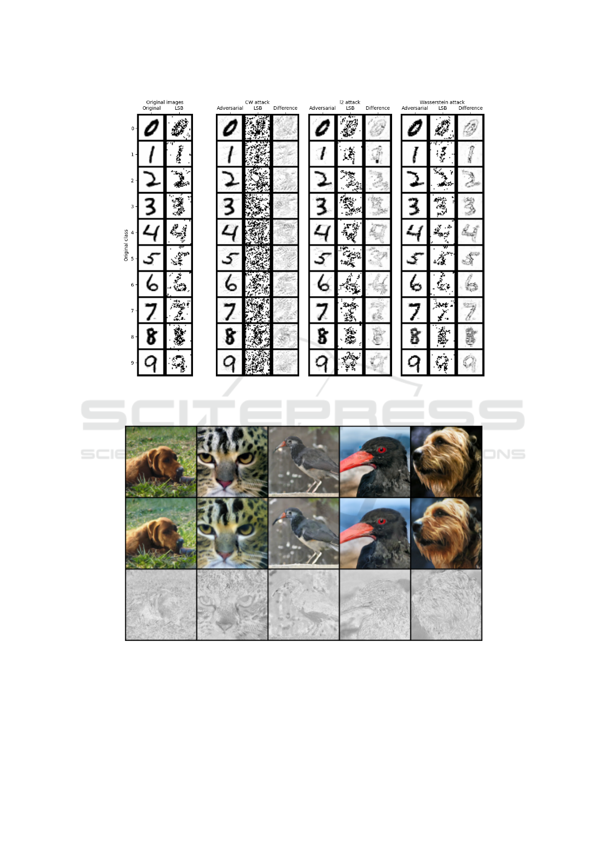
Figure 4: Comparison of CW and our attacks. Least significant bit (LSB) is defined in (9), the difference is between the
original and adversarial images. The figure shows that our attacks keep the hidden structure of the data (LSB) and that the
perturbations are not located randomly but around edges.
Figure 5: Unperturbed image (top), perturbed image (middle) and their difference (bottom). The perturbations happen around
key animal features.
the absolute pixel difference across all channels. This
difference shows interpretable silhouettes, which al-
lows us to assign semantical meaning to many per-
turbations. Most of the differences are concentrated
in key components of the animals, such as changes
of texture, colouring and brightness of their semanti-
cally meaningful components. For example, the dog
fur has a different texture, and the grass has lighter
colour. Another example is the bird’s beak, which is
longer in the third and thicker in the fourth adversar-
Adversarial Examples by Perturbing High-level Features in Intermediate Decoder Layers
503

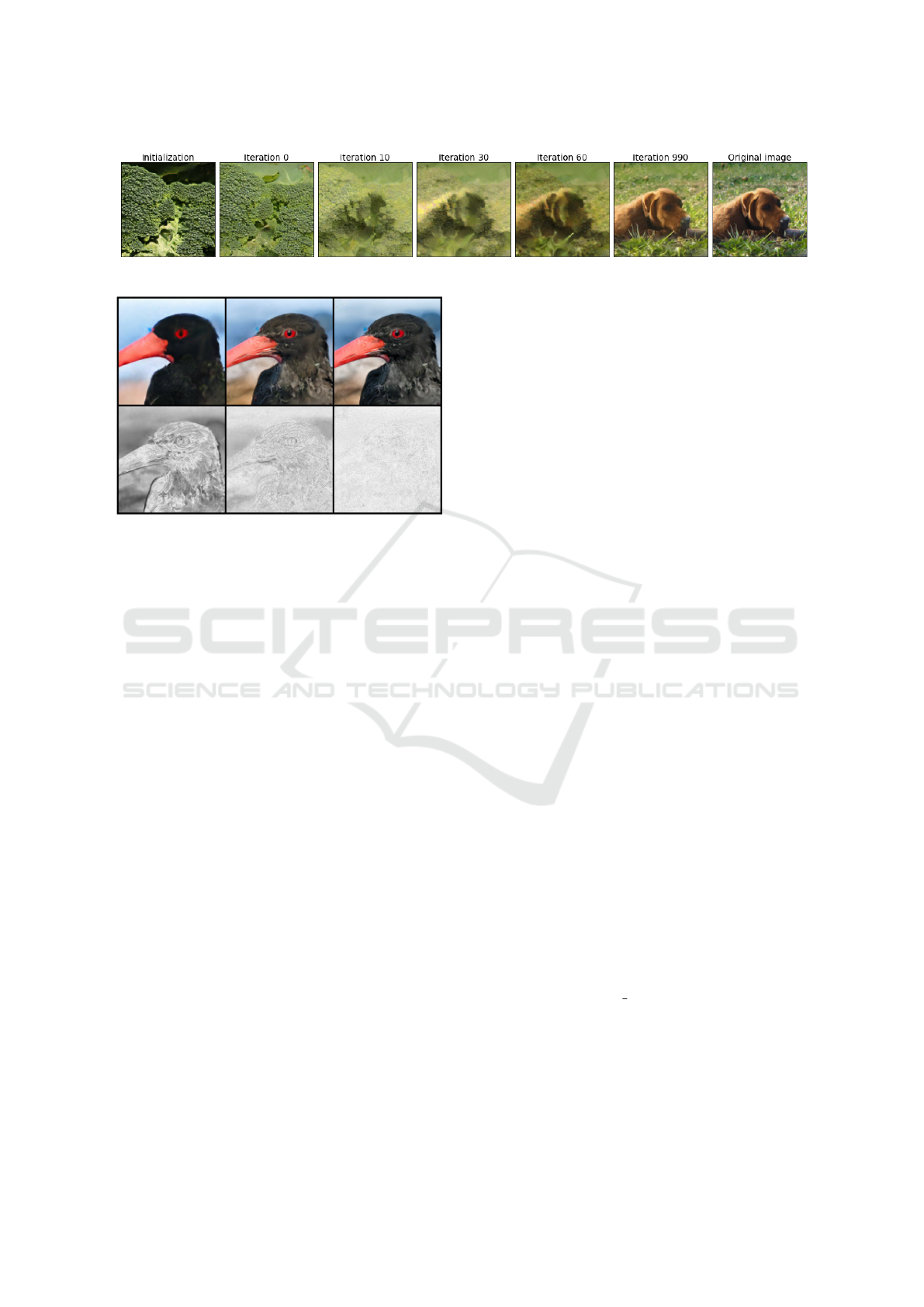
Figure 6: Development of perturbed images over iterations. Broccoli features get gradually incorporated into the dog.
Figure 7: Effect of the intermediate layer choice. The
columns show the perturbation in the first (left), second
(middle) and third (right) intermediate layer.
ial image. The difference plot also shows that signif-
icant perturbations happen around animals edges or
key features such as eyes and nose.
The crucial idea of our paper is to perturb the in-
termediate decoder layers. However, we can place
the perturbation in any intermediate layer, each with
a different effect. The earlier layers generate high-
level features, while later layers generate much finer
features or even perturbations in pixels without any
semantic meaning. Figure 7 shows the impact of the
choice of the intermediate layer. The columns show
the adversarial images when perturbing the first (left
column), second (middle column) and third (right col-
umn) intermediate layer. The figure shows that the
deeper we perturb the decoder, the more the perturba-
tions shift from high-level to finer perturbations. The
first layer results in a purely black bird and uniform
background. The silhouettes show that while the first
layer perturbs the colour of the chest, the beak or the
background, the silhouette in the third layer disap-
pears, and the perturbations amount almost to pixel
perturbations.
Figure 6 documents a similar effect of high-level
perturbations. While the previous figure showed the
dependence of high-level features on the intermedi-
ate layer choice, this figure shows this dependence
on the development of iterations in Algorithm 1. The
left image shows the broccoli image used for the ini-
tialization of our algorithm. The right image shows
the unperturbed dog. The middle five images visual-
ize how the perturbations modify the broccoli image
as the number of iterations increases. At the begin-
ning of the algorithm run, the perturbations are inter-
pretable: the dog is reconstructed by high-level broc-
coli features. As the algorithm gradually converges,
the perturbed image increasingly resembles the origi-
nal dog as the broccoli features fuse with the dog im-
age. Some of the original broccoli features remain
integrated into the final adversarial image. For exam-
ple, the next-to-last picture contains a slightly lighter
green shade than the original dog picture. Similarly,
we can interpret the changes in the dog fur and muzzle
textures as they originate from the broccoli texture.
We point out that all central images are classified as
broccoli due to the construction of our algorithm.
6 CONCLUSION
This paper presented a novel method for generat-
ing adversarial images. Instead of the standard pixel
perturbation, we use an encoder-decoder model and
perturb high-level features from intermediate decoder
layers. Our method generates high-quality adversarial
images in both targeted and untargeted settings on the
MNIST and ImageNet datasets. Since our adversarial
images perturb high-level features, they are more re-
silient to being recognized as adversarial by standard
defence techniques.
ACKNOWLEDGEMENTS
This material is based upon work supported by, or
in part by, the Army Research Laboratory and the
Army Research Office under grant number W911NF-
20-1-0197. The authors acknowledge the sup-
port by the project Research Center for Informatics
(CZ.02.1.01/0.0/0.0/16 019/0000765).
REFERENCES
Brendel, W., Rauber, J., and Bethge, M. (2018). Decision-
based adversarial attacks: Reliable attacks against
ICAART 2022 - 14th International Conference on Agents and Artificial Intelligence
504

black-box machine learning models. In Inter-
national Conference on Learning Representations
(ICLR) 2018.
Carlini, N. and Wagner, D. (2017). Towards evaluating the
robustness of neural networks. In 2017 IEEE Sympo-
sium on Security and Privacy (SP), pages 39–57.
Chen, J., Jordan, M. I., and Wainwright, M. J. (2020). Hop-
skipjumpattack: A query-efficient decision-based at-
tack. In 2020 IEEE Symposium on Security and Pri-
vacy (SP), pages 1277–1294.
Cuturi, M. (2013). Sinkhorn distances: Lightspeed com-
putation of optimal transport. In Advances in Neural
Information Processing Systems 26, volume 26, pages
2292–2300.
Deng, J., Dong, W., Socher, R., Li, L.-J., Li, K., and Fei-Fei,
L. (2009). Imagenet: A large-scale hierarchical image
database. In 2009 IEEE conference on computer vi-
sion and pattern recognition, pages 248–255.
Donahue, J., Kr
¨
ahenb
¨
uhl, P., and Darrell, T. (2016).
Adversarial feature learning. arXiv preprint
arXiv:1605.09782.
Donahue, J. and Simonyan, K. (2019). Large scale adver-
sarial representation learning. In Advances in Neu-
ral Information Processing Systems, volume 32, pages
10541–10551.
Dumoulin, V., Belghazi, I., Poole, B., Mastropietro, O.,
Lamb, A., Arjovsky, M., and Courville, A. (2016).
Adversarially learned inference. arXiv preprint
arXiv:1606.00704.
Feydy, J., S
´
ejourn
´
e, T., Vialard, F.-X., Amari, S.-i., Trouve,
A., and Peyr
´
e, G. (2019). Interpolating between op-
timal transport and mmd using sinkhorn divergences.
In The 22nd International Conference on Artificial In-
telligence and Statistics, pages 2681–2690.
Goodfellow, I. J., Shlens, J., and Szegedy, C. (2015). Ex-
plaining and harnessing adversarial examples. In In-
ternational Conference on Learning Representations
(ICLR) 2015.
Johnson, N. F. and Jajodia, S. (1998). Exploring steganog-
raphy: Seeing the unseen. Computer, 31(2):26–34.
Kurakin, A., Goodfellow, I., and Bengio, S. (2016). Ad-
versarial machine learning at scale. arXiv preprint
arXiv:1611.01236.
LeCun, Y., Cortes, C., and Burges, C. (2010). Mnist hand-
written digit database. ATT Labs [Online]. Available:
http://yann.lecun.com/exdb/mnist, 2.
Madry, A., Makelov, A., Schmidt, L., Tsipras, D., and
Vladu, A. (2018). Towards deep learning models re-
sistant to adversarial attacks. In International Confer-
ence on Learning Representations (ICLR) 2018.
Meng, D. and Chen, H. (2017). Magnet: A two-pronged
defense against adversarial examples. In Proceedings
of the 2017 ACM SIGSAC Conference on Computer
and Communications Security, pages 135–147.
Nocedal, J. and Wright, S. (2006). Numerical optimization.
Springer Science & Business Media.
Papernot, N., McDaniel, P., Jha, S., Fredrikson, M., Celik,
Z. B., and Swami, A. (2016). The limitations of deep
learning in adversarial settings. In 2016 IEEE Euro-
pean Symposium on Security and Privacy (EuroS&P),
pages 372–387.
Rauber, J., Zimmermann, R., Bethge, M., and Brendel, W.
(2020). Foolbox Native: Fast adversarial attacks to
benchmark the robustness of machine learning models
in PyTorch, TensorFlow, and JAX. Journal of Open
Source Software, 5(53):2607.
Samangouei, P., Kabkab, M., and Chellappa, R. (2018).
Defense-gan: Protecting classifiers against adver-
sarial attacks using generative models. In Inter-
national Conference on Learning Representations
(ICLR) 2018.
Simonyan, K. and Zisserman, A. (2015). Very deep con-
volutional networks for large-scale image recognition.
In International Conference on Learning Representa-
tions (ICLR) 2015.
Song, Y., Shu, R., Kushman, N., and Ermon, S. (2018).
Constructing unrestricted adversarial examples with
generative models. In Advances in Neural Information
Processing Systems, volume 31, pages 8312–8323.
Szegedy, C., Zaremba, W., Sutskever, I., Bruna, J., Erhan,
D., Goodfellow, I., and Fergus, R. (2014). Intriguing
properties of neural networks. In International Con-
ference on Learning Representations (ICLR) 2014.
Tan, M. and Le, Q. V. (2019). Efficientnet: Rethink-
ing model scaling for convolutional neural networks.
In International Conference on Machine Learning,
pages 6105–6114.
Wong, E., Schmidt, F. R., and Kolter, J. Z. (2019). Wasser-
stein adversarial examples via projected sinkhorn it-
erations. In International Conference on Machine
Learning, pages 6808–6817.
Xiao, C., Li, B., yan Zhu, J., He, W., Liu, M., and Song,
D. (2018). Generating adversarial examples with ad-
versarial networks. In Proceedings of the Twenty-
Seventh International Joint Conference on Artificial
Intelligence, pages 3905–3911.
APPENDIX: ADDITIONAL
RESULTS
This section extends the results from the main
manuscript body. We will always present a figure and
then compare it with the corresponding figure from
the manuscript body. The former figures start with a
letter while the latter figures with a digit.
Figure 8 shows the untargeted attacks for the non-
robust network. It corresponds to Figure 3 from the
manuscript body. The images are again nice, with the
Wasserstein attack performing better than the l
2
at-
tack. The small digit in each subfigure shows to which
class the digit was misclassified. As we have already
mentioned, our method always works with feasible
points and, therefore, all digits were successfully mis-
classified. In other words, these images were gener-
ated randomly without the need for manual selection.
Adversarial Examples by Perturbing High-level Features in Intermediate Decoder Layers
505

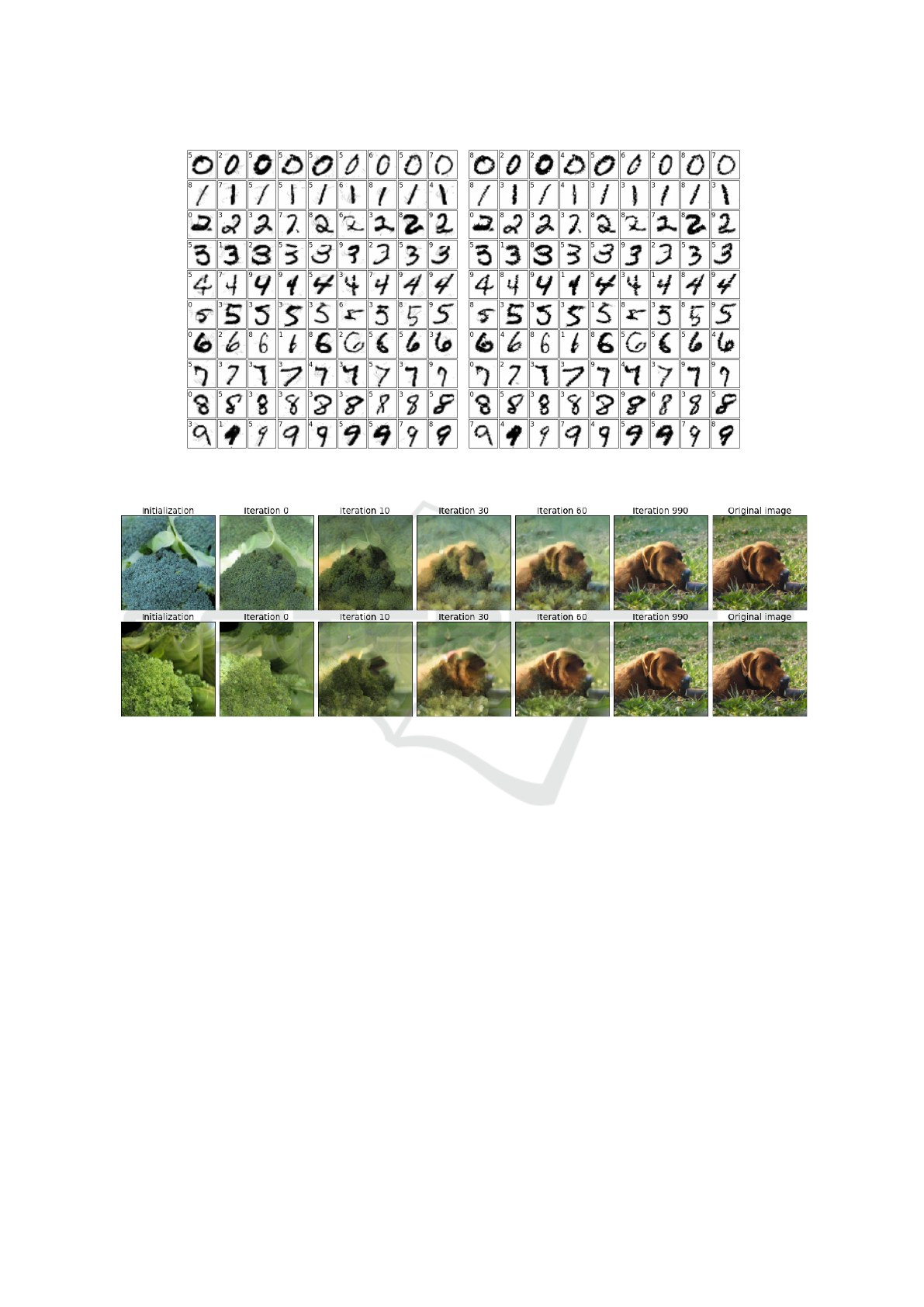
Figure 8: Untargeted l
2
attacks (left) and Wasserstein attacks (right). Rows represent the class. The small number in each
subfigure shows to which class the digit was classified.
Figure 9: Development of perturbed images over iterations. Broccoli features get gradually incorporated into the dog.
Figure 10 shows the attacks on the robust network
of (Madry et al., 2018). It corresponds to Figure 4
from the main manuscript body. The quality of the
CW attack increased. It now preserves the least sig-
nificant bit structure, and the perturbations shifted to-
wards the digit edges. The Wasserstein attack keeps
the superb performance with visually the same results
as in Figure 4. We conclude that our attacks are effi-
cient against adversarially trained networks.
Figure 11 shows the effect of the choices of the in-
termediate layer to perturb and of the initial point for
Algorithm 1. It corresponds to Figure 7 from the main
manuscript body. The first column shows the point
which was used to initialize Algorithm 1. The next
three columns present the adversarial images with the
perturbation inserted in different intermediate layers.
The last column shows the original image. The effect
of the initialization is negligible when perturbing the
third intermediate layer (column 4). However, it has
a huge impact when perturbing earlier intermediate
layers. The intermediate latent representation of the
second broccoli (rows 2 and 4) carries a preference
for the white colour, which is visible in the adversar-
ial image for the first intermediate layer (column 2).
Figure 9 also shows the effect of the initial point
for Algorithm 1. It corresponds to Figure 6 from the
main manuscript body. We see that the features of the
initial broccoli (column 1) gradually incorporate into
the dog image (columns 2-5). The adversarial image
(column 6) still have some connection to the initial
broccoli, for example, in the background colour. The
adversarial image is close to the original image (col-
umn 7). This figure shows that our algorithm works
with high-level features and not pixel modifications.
ICAART 2022 - 14th International Conference on Agents and Artificial Intelligence
506

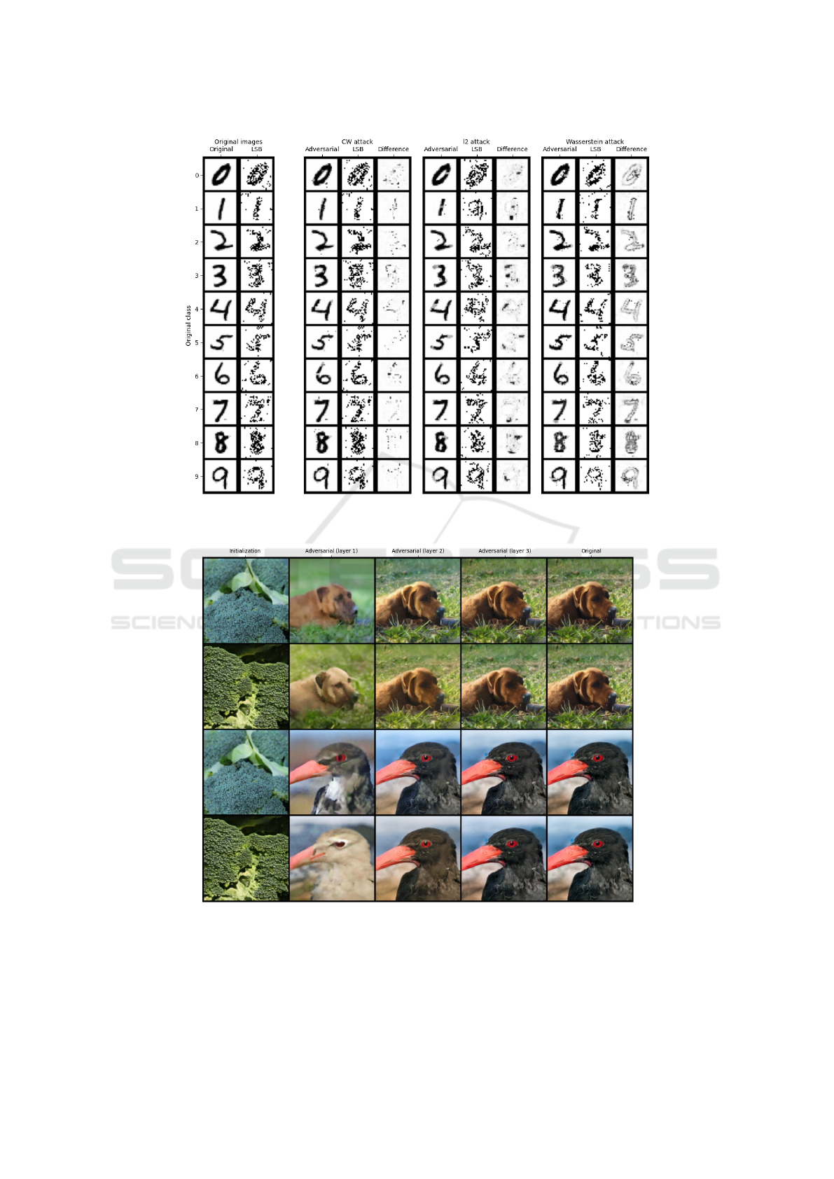
Figure 10: Comparison of CW and our attacks on the robust network. Least significant bit (LSB) is defined in (9), the
difference is between the original and adversarial images.
Figure 11: Effect of the intermediate layer choice. The columns show initial point for Algorithm 1 (column 1), the adversarial
image when perturbations were performed in the first (column 2), second (column 3) and third (column 4) intermediate layer
and the original image (column 5).
Adversarial Examples by Perturbing High-level Features in Intermediate Decoder Layers
507