Bone Segmentation of the Human Body in Computerized

Tomographies using Deep Learning

Angelo Antonio Manzatto

, Edson José Rodrigues Justino

and Edson Emílio Scalabrin

Programa de Pós Graduação em Informática, PPGIa - PUCPR, Curitiba, Paraná, Brazil

Keywords: Deep Learning, Medical Segmentation, Computed Tomography, Bones.

Abstract: The segmentation of human body organs in medical imaging is a widely used process to detect and diagnose

diseases in medicine and to help students learn human anatomy in education. Despite its significance,

segmentation is time consuming and costly because it requires experts in the field, time, and the requisite

tools. Following the advances in artificial intelligence, deep learning networks were employed in this study

to segment computerized tomography images of the full human body, made available by the Visible Human

Project (VHP), which included among 19 classes (18 types of bones and background): cranium, mandible,

clavicle, scapula, humerus, radius, ulna, hands, ribs, sternum, vertebrae, sacrum, hips, femur, patella, tibia,

fibula, and feet. For the proposed methodology, a VHP male body tomographic base containing 1865 images

in addition to the 20 IRCAD tomographic bases containing 2823 samples were used to train deep learning

networks of various architectures. Segmentation was tested on the VHP female body base containing 1730

images. Our quantitative evaluation of the results with respect to the overall average Dice coefficient was

0.5673 among the selected network topologies. Subsequent statistical tests demonstrated the superiority of

the U-Net network over the other architectures, with an average Dice of 0.6854.

1 INTRODUCTION

Segmentation in medical imaging is a crucial area

both within medicine, assisting in the identification

and treatment of diseases, and in education, teaching

students about the anatomy of the human body using,

for example, a digital anatomy table with such

capability while examining the tomography set from

a patient (Brongel et al, 2019). Recent studies, such

as those of Hesamian et al., (2019), have shown that

the performance achieved by deep learning networks

in image segmentation is superior to that of other

existing methods, leading to an impressive increase in

research efforts aimed at developing new and more

promising architectures in this area.

In medicine, studies have primarily focused on the

detection, prevention, and combat of serious diseases.

Research highlights with regard to deep learning

networks include segmentation of the computerized

tomography (CT) scans of the lungs ((Chunran and

Yuanyuan, 2018), (Shaziya et al, 2018), (Huang et al,

https://orcid.org/0000-0002-6263-1399

https://orcid.org/0000-0001-9145-6879

https://orcid.org/0000-0002-3918-1799

2018), (Kumar et at, 2019), (Alves et al, 2018), (Jin

et al, 2017), (Gerard and Reinhardt, 2019)), with the

purpose of detecting pulmonary nodules to fight lung

cancer as well as segmentation of the CT images of

the liver ((Jiang et al, 2019), (Wang et al, 2019),

(Shrestha and Salari, 2018), (Ahmad et al, 2019),

(Wang et al, 2019), (Chen et al, 2019), (Li et al,

2018), (Rafiei et al, 2018), (Xia et al, 2019). (Truong

et al, 2018), (Zhou et al, 2019)), both to track tumors

and lesions, and to aid in preoperative activities.

Other studies directly applicable to the medical field

and linked to the use of deep learning networks

include segmentation of the brain surface in post-

surgical activities of epilepsy patients ((Shell and

Adam, 2020)), segmentation of the esophagus for

cancer treatment ((Chen et al, 2019), (Trullo et al,

2017), (Trullo et al, 2017)), and segmentation of the

spine ((Fang et al, 2018), (Tang et al, 2019), (Kuok et

al, 2018)) to assist in pre-surgical activities.

In the course of the evolution of deep learning

networks, a few studies have thoroughly tested the

Manzatto, A., Justino, E. and Scalabrin, E.

Bone Segmentation of the Human Body in Computerized Tomographies using Deep Learning.

DOI: 10.5220/0010891200003182

In Proceedings of the 14th International Conference on Computer Supported Education (CSEDU 2022) - Volume 2, pages 17-26

ISBN: 978-989-758-562-3; ISSN: 2184-5026

limits of a single network segmenting all body organs

for the possible creation of a medical atlas. A 3D deep

learning network model/architecture, trained in a

semi-supervised manner combining supervised

learning using a small amount of labelled data with

unsupervised learning on massive unlabelled data,

was proposed to segment 16 abdominal organs (Zhou

et al, 2019). The use of a U-Net type deep learning

network was also proposed for the computerized

segmentation of six different types of bones (La Rosa,

2017). The lack of complete body tomographic image

bases and the lack of available specialists to create

ground truth masks of segmented images for each

organ have been a major impediment to advances

toward the creation of a medical atlas.

To advance along this direction, in this paper, we

present the results of segmenting one of the most

complete tomographic bases in the world, the Visible

Human Project (VHP), into 19 classes using deep

learning networks, with 18 of the classes denoting 18

different bones, and one class denoting the

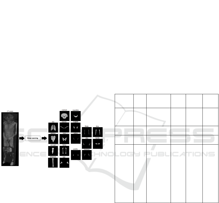
background, as illustrated in Figure 1.

Figure 1: Segmentation of a CT image base into 18 bone

classes. The images were extracted from the VHP male

database and compiled by the author.

Five network topologies were selected to perform

the segmentation task: U-Net, DenseNet, ResNet,

DeepLab, and FCN; all of which were trained in the

supervised mode. The Dice coefficient was used as a

metric to evaluate the results. Statistical tests such as

ANOVA and the non-parametric post-hoc Games-

Howell test were used to compare the performances

of the five different architectures of deep learning

networks in question.

The remainder of this paper is organized as

follows. Section 2 presents studies related to bone

segmentation using deep learning networks. Section

3 describes the method used both in the creation of

the ground truth bases and in the training, testing, and

analysis of the segmentation results. Section 4

presents an analysis of the results and discussion.

Section 5 concludes by highlighting the main results

and proposals for future research.

2 RELATED WORK

Three studies ((Fang et al, 2018), (Kuok et al, 2018),

(La Rosa, 2017)) with focus on the application of

deep learning networks to bone segmentation were

chosen to compare against. Some characteristics of

the items common to all these research studies were

compared against those of the current study. Table 1

shows the size of the databases used for training,

number of bone classes to be segmented, and metrics

for measuring the performance of the deep learning

networks pertaining to these studies.

Table 1: Deep learning networks specifically for bone

segmentation.

Reference

Qty.

classes

Bone classes

Qty

Training

Base

Network Metric

La Rosa, F.

(2017)

vertebrae,

sacrum, hips,

ribs, femur,

and sternum

15653 U-Net Dice

Kuok et al.

(2018)

1 vertebrae 200 DenseNet Dice

Fang et al.

(2018)

1 vertebrae 4500 FCN Accuracy

This article 18

cranium,

mandible,

clavicle,

scapula,

humerus,

radius, ulna,

hands, ribs,

sternum,

vertebrae,

sacrum, hips,

femur, patella,

tibia, fibula,

and feet

4688

(Male

VHP +

IRCAD

bases)

U-Net,

DenseNet,

ResNet,

DeepLab

and FCN

Dice

Although La Rosa uses a base containing 15653

samples to train a single U-Net for the segmentation

of six classes of bones of the abdominal region, in this

study, we used multiple bases for a total of 4688

(1865 male VHP + 2823 IRCAD) training samples,

which were segmented into 18 classes. An additional

test base (1730 female VHP), which represented a

significant challenge in terms of volume of

experiments, was used to evaluate five distinct

network topologies. The only class common to the

aforementioned studies was the vertebra, and as noted

earlier, the Dice metric was the predominant metric

for performance measurement. Although the three

studies sought to achieve the best segmentation by

CSEDU 2022 - 14th International Conference on Computer Supported Education

training a deep learning network topology, here in

addition to segmentation, we investigate whether

there is a significant difference in the segmentation

results among the five different deep learning

network topologies, using statistical analysis.

3 METHOD

The experimental method is structured as follows:

database selection, creation of ground truth base,

definition of deep learning network topologies,

supervised training of deep learning networks, cross-

validation, and collection and statistical analyses of

the results.

3.1 Databases

Two different tomographic image databases were

selected for experimentation: the first database

provided by the National Library of Medicine, is

referred to as the Visible Human Project (VHP)

, and

the second database provided by the Institute for

Research Against Digestive Cancer (IRCAD)

The selection of the VHP database was because of

its uniqueness, in that it consisted of full-body CT

scans, allowing us to explore the challenges of

segmenting all types of different bones, a challenge

not put into practice in other works ((Fang et al,

2018), (Kuok et al, 2018), (La Rosa, 2017)). These

studies focused on one type of bone or a single area

of the body, such as the abdominal region. The

IRCAD database was selected to complement the

model training database because it has segmentation

of the bones in the abdominal region.

The VHP Project image base includes two

tomographic sets: male and female. The male body

base contains 1865 512 × 512 pixel copies, whereas

the female human body base contains 1730 512 × 512

pixel copies. The database provided by IRCAD

consists of 2823 512 × 512 pixel CT images from 20

clinical studies, involving lesions and tumors of

various patients, anonymized in DICOM format. In

conducting the experiments, we segregated the

datasets into two groups: S1 and S2. Set S1,

exclusively used for training, contains the VHP male

database plus the 20 IRCAD databases, totaling 4688

images. In contrast, group S2 contains only the

female VHP database intended for testing, data

collection, and results analysis to verify the

https://www.nlm.nih.gov/research/visible/visible_human.

html

https://www.ircad.fr/research/3d-ircadb-01/

generalization power of the segmentation on a base

other than the one used during training. In the pre-

processing step, all images from the VHP and IRCAD

bases were converted to 8-bit monochrome color

scale with grayscales ranging from 0 to 255 and saved

in PNG format.

The procedure adopted in the preparation of each

ground truth mask for the 18 bone classes consisted

of applying: (a) thresholding layers to each

tomographic image to eliminate a significant part of

the background and other organs, and (b) using

different combinations of selection tools to segment

each bone class and subsequently create a binary

image in PNG format for the generation of the mask.

This procedure was applied to all 6418 CT images,

generating a total of 14 602 masks, as shown in Table

2 and took approximately eight months to complete.

Table 2: Number of ground truth masks of bone class in the

Visible Human Project male and female human body bases

along with the 20 IRCAD bases.

The entire manual segmentation process for the

creation of the ground truth was performed only by

the first author of this article, using a CT scan

specialist at CETAC (Centro de Tomografia

Computadorizada LTDA) in the city of Curitiba

(Brazil) and a medical atlas (Fleckenstein and

Tranum-Jensen, 2018) in case of doubts.

Our dataset is publicly available for download at the

following link: https://www.ppgia.pucpr.br/datasets/SA/

Classes Male VHP VHP female IRCAD

clavicle 94 86 17

craniu

174 160 0

feet 152 162 0

femu

486 423 42

fibula 401 345 0

hands 143 167 0

hips 219 213 255

humerus 240 280 12

mandible 106 82 0

atella 52 52 0

radio 129 216 0

ribs 390 366 1929

sacru

157 127 65

scapula 176 164 100

sternu

210 188 407

tibia 410 351 0

ulna 146 198 0

vertebrae 619 598 2707

Total 4304 4178 5534

Bone Segmentation of the Human Body in Computerized Tomographies using Deep Learning

3.2 Network Topologies

Five topologies of deep learning networks were

chosen for the study: U-Net, DenseNet, ResNet,

DeepLab, and FCN. As each network can be

assembled in countless ways and encompass an

infinite number of variations, we selected

architectures already discussed in image

segmentation related manuscripts. Some changes

were introduced to adapt the topologies to the

proposal of this work, such as accepting a 512 × 512

× 1 tensor (height, width, and depth) monochrome

computed tomography image as input and producing

a 512 × 512 × 19 tensor (height, width, and number

of classes, 18 bones and the background) for output,

referred to as the resulting segmentation.

Figure 2: Topology of the U-Net network.

The U-Net network architecture (Figure 2), of

Ronneberger et al., (2015), consists of a contraction

part and an expansion part. Each path of the

contraction contains two blocks formed by a 3 × 3

convolution layer without padding, followed by an

activation layer resembling a rectifier linear unit

(ReLU), and a 2 × 2 max pooling contraction layer.

The number of filters is doubled after each

contraction block following the sequence of 64, 128,

256, 512, and 1024 filters to the deepest level while

halving the number of filters at each expansion block.

Expansion blocks are created by upsampling or by

concatenating 2 × 2 transposed convolution layers to

the output along with the features of the appropriate

contraction layer. A 1 × 1 convolution layer is applied

at the end to go from a multidimensional space of 64

to a monochrome image.

To conserve space, only a very brief description

of the other topologies is presented. The DenseNet

topology was implemented using the FC-

DenseNet103 model (Jegou et al, 2017), which deals

with semantic segmentation issues. The ResNet

architecture was implemented as described in

(Liciotti et al, 2018), where the original version was

applied to the task of people tracking crowded

environments through aerial view images. ResNet

deals with the vanishing/exploding gradient problem

in which the network weights are practically zero or

tend to infinite values when the network has multiple

layers, introducing the concept of shortcut

connection.

The DeepLab topology was implemented using

the DeepLab V3 Plus model (Chen et al, 2018). In

addition to depthwise separable convolution layers

(Chollet, 2017), the model includes a refinement in

the decoder part of the architecture, allowing the use

of convolutional layers with upsampling, referred to

as atrous convolution, which solves the problem of

loss of resolution in the multiple layers resulting from

downsampling during convolution or pooling with a

stride greater than one. The model also employs a

process called atrous spatial pyramid pooling

(ASPP), in which the fusion of multiple atrous

convolution layers with different sampling rates is

applied to the input image, allowing the capture of

features at different scales of the objects to be

segmented.

A fully convolutional network (FCN) topology

has also been implemented as described in

(Shelhamer et al, 2017). Here the VGG16 topology

(Simonyan and Zisserman, 2015) constitutes the body

of the encoder part and the output segmentation is

refined by concatenating the deconvolution layers

with the max pooling layers.

All the aforementioned networks had their last

convolutional layer adapted to generate an output

tensor of size 512 × 512 × 19 pixels before passing

through a Softmax-type activation layer.

3.3 Training and Collection of Results

Figure 3 presents the general scheme of the

experiments, which consists of four steps. Each of the

five networks were subjected to a training process to

obtain the segmentation model (step 1). As the next

step, each model was used to segment the

tomographic image base of test S2 (step 2). A

statistical analysis was carried out on the results to

evaluate the quality of the segmentation. The number

of true positive (TP), true negative (TN), false

positive (FP), and false negative (FN) were

determined for each channel of the network output

segmented image in relation to the corresponding

class in the ground truth image. The statistics were

subsequently used to calculate the Dice coefficient as

an evaluation metric (step 3). The experiments were

concluded with a statistical analysis on the

performances of the five deep learning network

topologies in question vis-à-vis the VHP and IRCAD

image bases (step 4).

CSEDU 2022 - 14th International Conference on Computer Supported Education

Figure 3: Basic scheme of evaluation of deep learning

networks.

The training of the networks was performed using

a GPU with variable memory from 12 to 16 GB. The

software algorithms were programmed in Python

using the OpenCV and Matplotlib libraries for image

pre-processing and Keras for training and testing of

the deep learning networks. The number of network

parameters and layers as well as the average time

required to complete one training along with the batch

size for each network topology are listed in Table 3.

Table 3: Configuration parameters of the networks during

post-training of the experiments.

Network

Total

arameters

Layer Training time

Batch

Size

U-Net 31

053

965 73 27 h 43 min 20 s 4

DenseNet 9

426

355 494 35 h 13 min 20 s 2

ResNet 2,754

771 276 28 h 31 min 40 s 4

DeepLab 41

257

123 412 29 h 20 min 00 s 4

FCN 134

455

833 35 28 h 35 min 00 s 2

To avoid biased results, we used the cross-

validation method with five folds for each deep

learning network topology, using the following

protocol in each training session (Table 4):

Table 4: Training protocol of the experiments.

Parameters Value

Number of e

ochs 100

Trainin

base S1

(

male VHP + IRCAD

)

Trainin

/ Validation 80 % / 20 %

Weight optimization

orithm

Adam

Learnin

rate 0.0001

Batch size 2 or 4

Cost function Weighted Cross Entrop

Chance to apply data

augmentation per technique

for each sample

15%

Data augmentation

techniques

Rotation, translation, scaling,

horizontal mirroring, elastic

deformation, saturation,

contrast

The cost function for calculating the gradients, in

the process of updating the weights of each network,

is the weighted cross entropy (Equation 1):

𝐿



𝑙,𝑞



1

𝑀



𝑤









𝑥





𝑝







log



𝑝





𝑥





(1)

where M represents the number of pixels of the

segmented image; N is the number of classes; w

(x)

is the value of the class weight n applied to pixel x;

represents the value of the ground truth pixel; and

is the probability predicted by the Softmax layer

for the output of the deep learning network for pixel

To reduce the overfitting generated by the

unbalanced samples, different weights were applied

to the cost function (Equation 1) for each bone class.

Each weight was calculated using Equation 2, where

freq(c) is the pixel frequency of a given bone class

divided by the total number of pixels in all images in

which the class appears, and freq

is the median pixel

frequency of all classes, as displayed in Table 5.

𝛼





𝑓

𝑟𝑒𝑞



𝑓

𝑟𝑒𝑞



𝑐



(2)

Table 5: Weights assigned to each bone class for the

Weighted Cross Entropy cost function.

Class Weight

background 0.00033

clavicle 3.851657

cranium 0.189668

feet 0.681439

femur 0.236127

fibula 2.563772

hands 1.884704

hips 0.194719

humerus 1

mandible 1.740797

patella 6.942333

radio 6.094191

ribs 0.09294

sacrum 0.653063

scapula 1.145436

sternum 2.256164

tibia 0.431686

ulna 4.130787

vertebrae 0.041536

Bone Segmentation of the Human Body in Computerized Tomographies using Deep Learning

All weights were calculated prior to training

globally.

After each training, the data collection process

was performed in the S2 base by following the

sequential steps outlined below:

1-The trained network performs the segmentation of

the CT scan, obtaining an image consisting of 19

channels, 18 for the bone classes, and one for the

background.

2-With the ground truth mask for each of the 19

classes, the number of true positive (TP), true

negative (TN), false positive (FP), and false negative

(FN) were calculated.

3-The data calculated for each class were saved in a

line of the "csv" file with the first column having the

tomography identifier name, and the rest of the

information following the previously outlined steps in

Figure 3, for each class.

Twenty-five training runs were performed, that is,

five experiments for each of the following networks:

U-Net, DenseNet, ResNet, DeepLab, and FCN.

4 EXPERIMENTAL RESULTS

This section presents the results of the segmentation

of the CT scan images, as well as a three-dimensional

visualization of the segmentation of some of the bone

classes.

4.1 Bone Segmentation of the Human

Body

Segmentation on set S2 followed the training step

conducted on set S1 with 5-fold cross-validation. The

training and validation workflow were executed five

times for each network topology. The Dice

coefficient, or Sørensen-Dice, is given by Equation 3,

where TP was chosen as an evaluation metric to

compare the degree of similarity between the

segmentation output of the network and the ground

truth mask.

𝐷𝑖𝑐𝑒

2𝑇𝑃



𝐹𝑃



𝐹𝑁

(3)

There are several situations in which the presence

of the evaluated class simply does not exist in the

tomography, for example, the class "feet" or the class

"femur" when the head region is being evaluated. In

these cases, only true negative (TN) values are

acceptable as correct; however, the Dice coefficient

does not make an exception for these situations,

generating a division by zero. In such cases, one is not

sure whether the model predicted false correctly, by

way of learning or whether there is an overfitting

problem of the dominant class “background”.

Therefore, we decided to disregard the coefficient

measurements for each class outside the range of

images in which they do not appear. This implies that,

for the segmentation of the S2 base, of the generated

images with 19 channels totaling 32 870 masks, only

4178 were considered in the evaluation.

Table 6 presents the Dice coefficients calculated

from the S2 set, for the five network topologies: U-

Net, DenseNet, ResNet, DeepLab, and FCN. For each

topology, the average Dice coefficient was calculated

across the five individual trainings for each network

in the k-fold process, with k equal to five.

Table 6: Overall average of the Dice coefficients for each

class. The green color highlights the coefficients that

exceeded the value of 0.700.

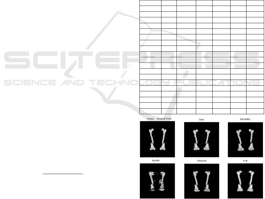
Figure 4: Segmentation of femur bones from the base of the

VHP female body for each network topology compared to

ground truth.

Dice U-Net DenseNet ResNe

DeepLab FCN Average

clavicle 0.7130 0.6744 0.4494 0.6468 0.5280 0.6023

cranium 0.8092 0.8170 0.7296 0.8239 0.6779 0.7715

feet 0.6475 0.3444 0.3062 0.3403 0.5878 0.4452

femu

0.8761 0.7748 0.6718 0.8298 0.7435 0.7792

fibula 0.7368 0.5357 0.4482 0.6728 0.5547 0.5896

hands 0.5411 0.4810 0.2125 0.2404 0.2676 0.3485

hips 0.7940 0.7433 0.6638 0.7609 0.7150 0.7354

humerus 0.6453 0.6575 0.4426 0.7285 0.5912 0.6130

mandible 0.7991 0.7559 0.6845 0.7961 0.6695 0.7410

patella 0.6951 0.7623 0.1798 0.2106 0.4704 0.4636

radio 0.3620 0.3700 0.3149 0.3926 0.3058 0.3491

ribs 0.5687 0.5701 0.4128 0.4984 0.4304 0.4961

sacrum 0.4957 0.4069 0.3294 0.3889 0.4931 0.4228

scapula 0.6489 0.5623 0.4200 0.5637 0.4774 0.5345

sternum 0.5355 0.5394 0.3072 0.5152 0.3405 0.4476

tibia 0.8051 0.7683 0.5648 0.7517 0.7195 0.7219

ulna 0.5122 0.5663 0.2978 0.5708 0.4133 0.4721

vertebrae 0.7710 0.6746 0.5727 0.7166 0.6563 0.6782

Global 0.6642 0.6113 0.4449 0.5804 0.5357 0.5673

CSEDU 2022 - 14th International Conference on Computer Supported Education

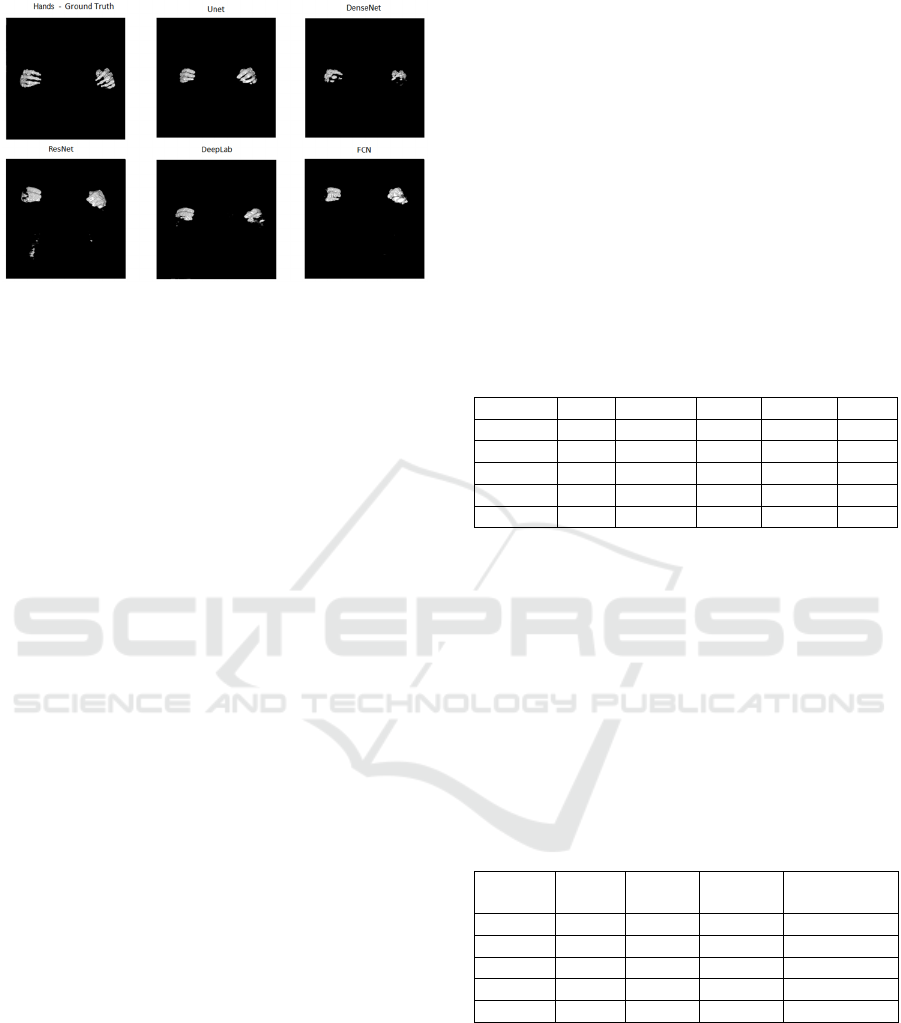
Figure 5: Segmentation of the bones of the hands from the

base of the female body of the VHP for each network

topology in comparison with the ground truth. It is observed

that there was practically no segmentation of the hand

bones by the networks.

In the images of Figures 4 and 5, it can be

observed that of among all bone classes, the

segmentation of the femur was the most successful,

as the femur Dice coefficient of 0.7729 was the

highest and the worst Dice coefficient of all bone

classes was the hand with a Dice coefficient of

0.3485. This finding can be observed in the

tridimensional images generated by each network.

Starting with the average Dice coefficients for

each deep learning network, calculated for the 4178

valid samples in set S2 and displayed in Table 6, we

performed several statistical tests using the IBM's

SPSS™ software to validate or refute the following

research hypotheses: Null Hypothesis H0: The

average Dice coefficient of all deep learning networks

are equal. Alternative Hypothesis H1: One of the

deep learning networks has at least one average Dice

coefficient that is different.

One-way analysis of variance (ANOVA) was

performed. Data normality was assessed using the

Kolmogorov-Smirnov and Shapiro-Wilk tests and

homogeneity of variance using Levene’s test.

Bootstrapping was also used with 1000 samples with

a reliability index (CI) of 95%, which increases the

confidence in the results obtained (Haukoos & Lewis,

2005). We also applied Welch correction on the

results and calculated the Dice coefficients to predict

the possibility of heterogeneity of variance in the

samples.

The preliminary results indicated that the samples

did not have a normal distribution (Kolmogorov-

Smirnov = 0.10, p-value < 0.001; Shapiro-Wilk =

0.95, p-value < 0.001), nor did they have

homogeneity of variance (Levene F(4, 20885), p-

value < 0.001). The results of ANOVA analysis of

variance, in contrast, showed that there is a

statistically significant difference between the means

of the Dice coefficients for the deep learning

networks [Welch's F(4, 10434.86) = 614.84, p-value

< 0.001], which refutes the null hypothesis H0 and

corroborates with the alternative hypothesis H1.

To find out which pairs of deep learning network

topologies show statistical differences, the non-

parametric post-hoc Games-Howell test was

performed, whereby it was found that only the deep

learning networks DenseNet and DeepLab were

similar (p-value = 0.8890 > 0.05), whereas all other

pairwise combinations were statistically different (p-

value < 0.01), as shown in Table 7.

Table 7: Games-Howell test shows that only the deep

learning networks DenseNet and DeepLab have statistical

similarity.

Finally, by analyzing the averages of the Dice

coefficients given in Table 8, it is observed that the

deep learning network U-Net has average Dice

coefficients significantly higher (0.6854) than those

of the other deep learning topologies analyzed. The

U-Net deep learning network performed the best in

the automatic segmentation of the VHP female body

as indicated by the Dice coefficients. It should also be

highlighted that U-Net has the second lowest variance

and standard deviation, and is the median with respect

to the number of parameters.

Table 8: Dice coefficient statistics on 4178 samples given

the number of training parameters.

etwor

Average Variance

Standard

Deviation

Parameters

U-Net 0.6854 0.0408 ±0.2021 31

053

965

DenseNet 0.6224 0.0475 ±0.2179 9

426

355

ResNet 0.4780 0.0417 ±0.2042 2

754

771

DeepLab 0.6270 0.0533 ±0.2308 41

257

123

FCN 0.5630 0.0394 ±0.1984 134

455

833

The box-and-whisker plot displayed in Figure 6

shows the distributions of the Dice coefficients for all

the female body CT images of the VHP or S2 set.

Such a graph allows visualization of the similarity

between the average Dice coefficient values of the

deep learning networks such as DenseNet and

DeepLab and the superior performance of the deep

learning network U-Net vis-à-vis the others alongside

P-value U-Net DenseNet ResNet Dee

Lab FCN

U-Net - 0.0000 0.0000 0.0000 0.0000

DenseNet 0.0000 - 0.0000 0.8890 0.0000

ResNet 0.0000 0.0000 - 0.0000 0.0000

DeepLab 0.0000 0.8890 0.0000 - 0.0000

FCN 0.0000 0.0000 0.0000 0.0000 -

Bone Segmentation of the Human Body in Computerized Tomographies using Deep Learning

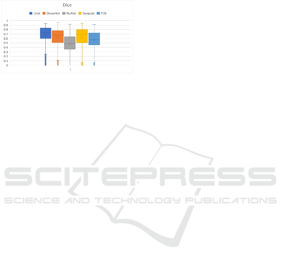
the low performance of the deep learning networks

ResNet and FCN.

Figure 6: Box-and-whisker plot for the Dice coefficient

associated with the performance of each deep learning

network used in the segmentation of tomographic images.

It is important to emphasize that the results

obtained depend on the topologies of the deep

learning networks assembled. The addition of extra

layers in the composition of each network can change

the results obtained. Therefore, generic conclusions

on each tested topology should be avoided.

5 CONCLUSIONS

In this study, we proposed the segmentation of a set

of male human body CT images from the Visible

Human Project (VHP) into 18 distinct bone classes

using deep learning networks by applying a workflow

consisting of the classical steps of: training, testing,

data collection, and pairwise statistical analysis. Until

the present moment of this paper we created the

largest ground truth bone dataset with respect to the

number of classes used in supervised training on a

medical segmentation task.

The results obtained by our tomographic image

segmentation experiments provided an overall

average Dice coefficient of 0.5673 for all classes of

segmented bones, considering the U-Net, DenseNet,

ResNet, DeepLab, and FCN networks together. The

main challenges were the limited number of

tomographic samples available for training, as well as

the great irregularity in the shape of the bones,

excessive presence of the "background" class, and

very close edges between bones of different classes.

Among the five U-Net, DenseNet, ResNet,

DeepLab, and FCN network topologies compared

using statistical tests, the U-Net topology

outperformed the others with a global average Dice

coefficient of 0.6854. DenseNet and DeepLab

networks exhibited slightly lower performance than

U-Net, but were statistically similar to each other,

with Dice coefficients of 0.6224 and 0.6270,

respectively. The FCN and ResNet topologies had the

worst performance with Dice coefficients of 0.5630

and 0.4780, respectively.

In future work, we will study more efficient

techniques that mitigate the influence of the

"background" class. We will also explore three-

dimensional topologies with 3D convolutional layers

and generative adversarial network networks. We will

examine techniques that allow the addition of new

classes from different databases without explicitly

changing the ground truth already produced. This

represents a stride towards the incremental

construction of an atlas of the human body containing

the segmentation of all organs using a single network

model.

REFERENCES

Brongel, A.; Brobouski, W.; Pierin, L.; Gomes, C.;

Almeida, M. and Justino, E. (2019). An Ultra-high

Definition and Interactive Simulator for Human

Dissection in Anatomic Learning.In Proceedings of the

11th International Conference on Computer Supported

Education - Volume 2: CSEDU, ISBN 978-989-758-

367-4, ISSN 2184-5026, pages 284-291. DOI:

10.5220/0007707102840291

Hesamian, M. H., Jia, W., He, X., & Kennedy, P. (2019).

Deep Learning Techniques for Medical Image

Segmentation: Achievements and Challenges. Journal

of Digital Imaging, 32(4), 582–596.

https://doi.org/10.1007/s10278-019-00227-x

Chunran, Y., & Yuanyuan, W. (2018). Nodule on CT

Images. 2–6.

Shaziya, H., Shyamala, K., & Zaheer, R. (2018). Automatic

Lung Segmentation on Thoracic CT Scans Using U-Net

Convolutional Network. Proceedings of the 2018 IEEE

International Conference on Communication and

Signal Processing, ICCSP 2018, 643–647.

https://doi.org/10.1109/ICCSP.2018.8524484.

Huang, C. H., Xiao, W. T., Chang, L. J., Tsai, W. T., & Liu,

W. M. (2018). Automatic tissue segmentation by deep

learning: From colorectal polyps in colonoscopy to

abdominal organs in CT exam. VCIP 2018 - IEEE

International Conference on Visual Communications

and Image Processing, 1–4. https://doi.org/10.1109/

VCIP.2018.8698645.

Kumar, A., Fulham, M., Feng, D., & Kim, J. (2019). Co-

Learning Feature Fusion Maps from PET-CT Images of

Lung Cancer. IEEE Transactions on Medical Imaging,

1–1. https://doi.org/10.1109/tmi.2019.2923601.

Alves, J. H., Neto, P. M. M., & Oliveira, L. F. (2018).

Extracting Lungs from CT Images Using Fully

Convolutional Networks. Proceedings of the

International Joint Conference on Neural Networks,

2018-July. https://doi.org/10.1109/IJCNN.2018.8489223.

CSEDU 2022 - 14th International Conference on Computer Supported Education

Jin, T., Cui, H., Zeng, S., & Wang, X. (2017). Learning

Deep Spatial Lung Features by 3D Convolutional

Neural Network for Early Cancer Detection. DICTA

2017 - 2017 International Conference on Digital Image

Computing: Techniques and Applications, 2017-

December, 1–6. https://doi.org/10.1109/DICTA.2017.

8227454.

Gerard, S. E., & Reinhardt, J. M. (2019). Pulmonary lobe

segmentation using a sequence of convolutional neural

networks for marginal learning. Proceedings -

International Symposium on Biomedical Imaging,

2019-April(Isbi), 1207–1211. https://doi.org/10.1109/

ISBI.2019.8759212.

Jiang, H., Shi, T., Bai, Z., & Huang, L. (2019). AHCNet:

An Application of Attention Mechanism and Hybrid

Connection for Liver Tumor Segmentation in CT

Volumes. IEEE Access, 7, 24898–24909.

https://doi.org/10.1109/ACCESS.2019.2899608

Wang, C., Song, H., Chen, L., Li, Q., Yang, J., Hu, X. T.,

& Zhang, L. (2019). Automatic Liver Segmentation

Using Multi-plane Integrated Fully Convolutional

Neural Networks. Proceedings - 2018 IEEE

International Conference on Bioinformatics and

Biomedicine, BIBM 2018, 518–523.

https://doi.org/10.1109/BIBM.2018.8621257

Shrestha, U., & Salari, E. (2018). Automatic Tumor

Segmentation Using Machine Learning Classifiers.

IEEE International Conference on Electro Information

Technology, 2018-May, 153–158. https://doi.org/10.

1109/EIT.2018.8500205

Ahmad, M., Ai, D., Xie, G., Qadri, S. F., Song, H., Huang,

Y., … Yang, J. (2019). Deep Belief Network Modeling

for Automatic Liver Segmentation. IEEE Access, 7,

20585–20595.

https://doi.org/10.1109/ACCESS.2019.2896961

Wang, Z. H., Liu, Z., Song, Y. Q., & Zhu, Y. (2019).

Densely connected deep U-Net for abdominal multi-

organ segmentation. Proceedings - International

Conference on Image Processing, ICIP, 2019-

September, 1415–1419. https://doi.org/10.1109/ICIP.

2019.8803103

Chen, X., Zhang, R., & Yan, P. (2019). Feature fusion

encoder decoder network for automatic liver lesion

segmentation. Proceedings - International Symposium

on Biomedical Imaging, 2019-April(Isbi), 430–433.

https://doi.org/10.1109/ISBI.2019.8759555

Li, X., Chen, H., Qi, X., Dou, Q., Fu, C. W., & Heng, P. A.

(2018). H-DenseU-Net: Hybrid Densely Connected U-

Net for Liver and Tumor Segmentation from CT

Volumes. IEEE Transactions on Medical Imaging,

37(12), 2663–2674. https://doi.org/10.1109/TMI.2018.

2845918.

Rafiei, S., Nasr-Esfahani, E., Soroushmehr, S. M. R.,

Karimi, N., Samavi, S., & Najarian, K. (2018). Liver

segmentation in ct images using three dimensional to

two dimensional fully convolutional network. ArXiv,

2067–2071.

Xia, K., Yin, H., Qian, P., Jiang, Y., & Wang, S. (2019).

Liver semantic segmentation algorithm based on

improved deep adversarial networks in combination of

weighted loss function on abdominal CT images. IEEE

Access, 7, 96349–96358. https://doi.org/10.1109/

ACCESS.2019.2929270

Truong, T. N., Dam, V. D., & Le, T. S. (2018). Medical

Images Sequence Normalization and Augmentation:

Improve Liver Tumor Segmentation from Small Data

Set. Proceedings - 2018 3rd International Conference

on Control, Robotics and Cybernetics, CRC 2018, 1–5.

https://doi.org/10.1109/CRC.2018.00010

Zhou, Y., Wang, Y., Tang, P., Bai, S., Shen, W., Fishman,

E. K., & Yuille, A. (2019). Semi-supervised 3D

abdominal multi-organ segmentation via deep multi-

planar co-training. Proceedings - 2019 IEEE Winter

Conference on Applications of Computer Vision,

WACV 2019, 121–140. https://doi.org/10.1109/

WACV.2019.00020.

Shell, Adam (2020), How to invest in artificial intelligence,

https://www.usatoday.com/story/money/2020/01/27/ar

tificial-intelligence-how-invest/4542467002/.

Chen, S., Yang, H., Fu, J., Mei, W., Ren, S., Liu, Y., …

Chen, H. (2019). U-Net Plus: Deep Semantic

Segmentation for Esophagus and Esophageal Cancer in

Computed Tomography Images. IEEE Access, 7,

82867–82877.

https://doi.org/10.1109/ACCESS.2019.2923760

Trullo, R., Petitjean, C., Ruan, S., Dubray, B., Nie, D., &

Shen, D. (2017). Segmentation of Organs at Risk in

thoracic CT images using a SharpMask architecture and

Conditional Random Fields. Proceedings -

International Symposium on Biomedical Imaging,

1003–1006.

https://doi.org/10.1109/ISBI.2017.7950685

Trullo, R., Petitjean, C., Nie, D., Shen, D., & Ruan, S.

(2017). Fully automated esophagus segmentation with

a hierarchical deep learning approach. Proceedings of

the 2017 IEEE International Conference on Signal and

Image Processing Applications, ICSIPA 2017, 503–

506. https://doi.org/10.1109/ICSIPA.2017.8120664

Fang, L., Liu, J., Liu, J., & Mao, R. (2018). Automatic

Segmentation and 3D Reconstruction of Spine Based

on FCN and Marching Cubes in CT Volumes. (2018)

10th International Conference on Modelling,

Identification and Control (ICMIC), (Icmic), 1–5.

Tang, Z., Chen, K., Pan, M., Wang, M., & Song, Z. (2019).

An Augmentation Strategy for Medical Image

Processing Based on Statistical Shape Model and 3D

Thin Plate Spline for Deep Learning. IEEE Access, 7,

133111–133121. https://doi.org/10.1109/ACCESS.

2019.2941154

Kuok, Chan-Pang and Hsue, Jin-Yuan and Shen, Ting-Li

and Huang, Bing-Feng and Chen, Chi-Yeh and Sun, Y.-

N. (2018). Segmentation from 3D CT Images. Pacific

Neighborhood Consortium Annual Conference and

Joint Meetings (PNC), (c), 1–6.

Zhou, Y., Wang, Y., Tang, P., Bai, S., Shen, W., Fishman,

E. K., & Yuille, A. (2019). Semi-supervised 3D

abdominal multi-organ segmentation via deep multi-

planar co-training. Proceedings - 2019 IEEE Winter

Conference on Applications of Computer Vision,

Bone Segmentation of the Human Body in Computerized Tomographies using Deep Learning

WACV 2019, 121–140. https://doi.org/10.1109/

WACV.2019.00020.

La Rosa, F. (2017). A deep learning approach to bone

segmentation in CT scans. 66. Retrieved from AMS

Laurea Institutional Thesis Repository.

P. Fleckenstein, J. Tranum-Jensen (2004), Anatomia em

Diagnóstico Por Imagens: 2. ed.,São Paulo: Manole,.

Ronneberger, O., Fischer, P., & Brox, T. (2015). U-Net:

Convolutional networks for biomedical image

segmentation. Lecture Notes in Computer Science

(Including Subseries Lecture Notes in Artificial

Intelligence and Lecture Notes in Bioinformatics),

9351, 234–241. https://doi.org/10.1007/978-3-319-

24574-4_28

Jegou, S., Drozdzal, M., Vazquez, D., Romero, A., &

Bengio, Y. (2017). The One Hundred Layers Tiramisu:

Fully Convolutional DenseNets for Semantic

Segmentation. IEEE Computer Society Conference on

Computer Vision and Pattern Recognition Workshops,

2017-July, 1175–1183. https://doi.org/10.1109/

CVPRW.2017.156

Liciotti, D., Paolanti, M., Pietrini, R., Frontoni, E., &

Zingaretti, P. (2018). Convolutional Networks for

Semantic Heads Segmentation using Top-View Depth

Data in Crowded Environment. Proceedings -

International Conference on Pattern Recognition,

2018-August, 1384–1389. https://doi.org/10.1109/

ICPR.2018.8545397

Chen, L. C., Zhu, Y., Papandreou, G., Schroff, F., & Adam,

H. (2018). Encoder-decoder with atrous separable

convolution for semantic image segmentation. Lecture

Notes in Computer Science (Including Subseries

Lecture Notes in Artificial Intelligence and Lecture

Notes in Bioinformatics), 11211 LNCS, 833–851.

https://doi.org/10.1007/978-3-030-01234-2_49

Chollet, F. (2017). Xception: Deep learning with depthwise

separable convolutions. Proceedings - 30th IEEE

Conference on Computer Vision and Pattern

Recognition, CVPR 2017, 2017-January, 1800–1807.

https://doi.org/10.1109/CVPR.2017.195

Shelhamer, E., Long, J., & Darrell, T. (2017). Fully

Convolutional Networks for Semantic Segmentation.

IEEE Transactions on Pattern Analysis and Machine

Intelligence, 39(4), 640–651. https://doi.org/10.1109/

TPAMI.2016.2572683

Simonyan, K., & Zisserman, A. (2015). Very deep

convolutional networks for large-scale image

recognition. 3rd International Conference on Learning

Representations, ICLR 2015 - Conference Track

Proceedings, 1–14.

Haukoos JS, Lewis RJ. Advanced statistics: bootstrapping

confidence intervals for statistics with "difficult"

distributions. Acad Emerg Med. 2005 Apr;12(4):360-5.

doi: 10.1197/j.aem.2004.11.018. PMID: 15805329.

CSEDU 2022 - 14th International Conference on Computer Supported Education