
Pose Guided Feature Learning for 3D Object Tracking on RGB Videos
Mateusz Majcher and Bogdan Kwolek
AGH University of Science and Technology, 30 Mickiewicza, 30-059 Krakow, Poland
Keywords:
3D Object Pose, Detection of Object Keypoints, Pose Tracking.
Abstract:
In this work we propose a new approach to 3D object pose tracking in sequences of RGB images acquired
by a calibrated camera. A single hourglass neural network that has been trained to detect fiducial keypoints
on a set of objects delivers heatmaps representing 2D locations of the keypoints. Given a calibrated camera
model and a sparse object model consisting of 3D locations of the keypoints, the keypoints in hypothesized
object poses are projected onto 2D plane and then matched with the heatmaps. A quaternion particle filter
with a probabilistic observation model that uses such a matching is employed to maintain 3D object pose
distribution. A single Siamese neural network is trained for a set of objects on keypoints from the current and
previous frame in order to generate a particle in the predicted 3D object pose. The filter draws particles to
predict the current pose using its a priori knowledge about the object velocity and includes the predicted 3D
object pose by the neural network in a priori distribution. Thus, the hypothesized 3D object poses are generated
using both a priori knowledge about the object velocity in 3D and keypoint-based geometric reasoning as well
as relative transformations in the image plane. In an extended algorithm we combine the set of propagated
particles with an optimized particle, whose pose is determined by Levenberg-Marguardt.
1 INTRODUCTION
Determining pose between object and camera is a
classical problem in computer vision, but it has re-
cently attracted considerable attention. Although
RGBD-based methods can estimate 6DoF object pose
with high accuracies on popular benchmark data
(Kaskman et al., 2019), considerable research efforts
are devoted to RGB-based methods for 3D object
pose estimation to improve their efficiency and usabil-
ity. The RGB-only approaches suffer heavily from in-
herent scale ambiguities (Xiang et al., 2018). Existing
methods can be divided into category level methods
(Pavlakos et al., 2017; Wang et al., 2018; Chen et al.,
2021) and instance level methods (Rad and Lepetit,
2017; Kehl et al., 2017; Tekin et al., 2018; Peng et al.,
2019; Hu et al., 2019). The former group encom-
passes methods that focus more on handling intra-
category variation and aims at estimating poses for an
entire category. In later methods, training set and test
set contain the same objects.
In general, recent methods follow either of two
approaches: (i) keypoint-based approaches that de-
tect a sparse set of keypoints and afterward align a
3D object representation to detections on the image,
(ii) rendering-based approaches utilizing a generative
model, that is built on a 3D mesh representation of an
object undergoing observation. The later methods es-
timate the object pose by reconstructing the input im-
age through rendering-and-comparing (analysis-by-
synthesis) and usually better cope with partial occlu-
sions (Egger et al., 2018).
Recent methods for object pose estimation are
based on convolutional neural networks (CNNs).
They can be divided into indirect and direct meth-
ods. Indirect methods aim at establishing 2D-3D
correspondences between the coordinates in the im-
age plane and object coordinates or learn a pose em-
bedding at an intermediate stage. In contrast, direct
methods determine the final 6D pose without using
such an intermediate representation. A first attempt
to utilize a CNN for direct regression of 6DoF ob-
ject poses was PoseCNN (Xiang et al., 2018). How-
ever, existing CNN-based methods usually need sep-
arate networks for each object instance (Kehl et al.,
2017; Tekin et al., 2018; Manhardt et al., 2020),
which results in long training times. The current top-
performing deep learning-based methods rely on the
indirect strategies. For instance, in (Rad and Lepetit,
2017) the 2D projections of fixed points, e.g. the 3D
corners of the encapsulating bounding box are deter-
mined. (Hu et al., 2019; Peng et al., 2019) addition-
ally perform object segmentation coupled with vot-
ing for each correspondence in order to improve the
574
Majcher, M. and Kwolek, B.
Pose Guided Feature Learning for 3D Object Tracking on RGB Videos.
DOI: 10.5220/0010886800003124
In Proceedings of the 17th International Joint Conference on Computer Vision, Imaging and Computer Graphics Theory and Applications (VISIGRAPP 2022) - Volume 5: VISAPP, pages
574-581
ISBN: 978-989-758-555-5; ISSN: 2184-4321
Copyright
c
2022 by SCITEPRESS – Science and Technology Publications, Lda. All rights reserved

performance and robustness. Most pf the recent re-
search efforts are directed towards predicting dense
rather than sparse correspondences (Zakharov et al.,
2019; Fan et al., 2021). There are also first attempts to
make RANSAC/PnP differentiable (Brachmann and
Rother, 2019).
Although, vast work has been done in the field
of 3D object pose estimation, there is comparatively
small number of related works on 3D object tracking
(Fan et al., 2021). Moreover, most existing methods
deliver only a single guess of the object’s pose. In
robotic applications, such approaches can be less use-
ful as robots should be aware of pose uncertainty be-
fore taking an action. Modeling uncertainties through
continuous distributions over 3D object coordinates
or bounding box coordinates have been studied in
(Brachmann et al., 2016) and (Tremblay et al., 2018),
respectively. Recently, (Majcher and Kwolek, 2021)
proposed deep quaternion pose proposals for 3D ob-
ject pose tracking on RGB images. A 3D object
model is rendered and then matched with the object
segmented in advance by a neural network. Object
keypoints detected by a simple neural network are fed
to PnP algorithm in order to calculate an object pose
hypothesis, which is then injected into the probability
distribution, recursively updated in a Bayesian frame-
work.
Inspired by the analysis above and gaps in existing
approaches, in this work we propose a novel approach
to 3D object pose tracking in sequences of RGB im-
ages acquired by a calibrated camera. We trained
a single hourglass neural network in order to detect
fiducial keypoints on a set of objects, which delivers
heatmaps representing 2D locations of the keypoints.
Given a calibrated camera model and a sparse object
model consisting of 3D locations of the keypoints,
the keypoints in hypothesized poses of the object are
projected onto 2D plane and then matched with the
heatmaps. A quaternion particle filter with probabilis-
tic observation model that uses such a matching is em-
ployed to maintain 3D object pose distribution. For a
set of objects, we also trained a single Siamese neu-
ral network on keypoints from the current and previ-
ous frame in order to generate a predicted object pose
on the basis of geometrical relations and motion of
the keypoints in the image plane. The filter draws
particles to predict the current pose using its a pri-
ori knowledge about the object velocity and includes
the predicted 3D object pose by the neural network in
a priori distribution. Owing to reliable detections of
object keypoints and heatmap-based representation of
keypoint locations, a simplified keypoint only-based
observation model has been proposed for a Bayesian
filter, which permits reliable tracking of 3D object
pose. The novelty of this work lies in synergistic
combination of 2D and 3D information about object
motion to generate object pose hypotheses, which are
then verified on the basis of deep heatmaps, deter-
mined by the learned neural network.
2 METHOD
At the beginning we outline quaternions and explain
the motion model of quaternion particle filter. In Sub-
section 2.2 we present a neural network for extracting
object keypoints. Subsection 2.3 details the algorithm
for 3D object pose tracking.
2.1 Quaternion Particle Filter
Quaternions can be viewed as numbers with one real
part and three distinct imaginary parts: q = q
w
+
q
x
i + q
y
j + q
z
k, where q
w
, q
x
, q
y
, and q
z
are real num-
bers, and i, j, k satisfy i
2
= j
2
= k
2
= ijk = −1, and
ij = −ji = k, jk = −kj = i, ki = −ik = j. This implies
that quaternion multiplication is generally not com-
mutative. The quaternion q = q
w
+q
x
i +q
y
j +q
z
k can
also be viewed as q = w+v, where v = q
x
i+q
y
j+q
z
k.
A unit-length quaternion (|q| = 1) is generated by
dividing each of the four components by the square
root of the sum of the squares of those components.
Every quaternion with unit magnitude enforces the
number of DoF to three, and thus represents a rota-
tion of angle θ about an arbitrary axis. Unit quater-
nions can be represented as a sphere of radius equal
to one unit. The vector originates at the sphere’s cen-
ter, and all rotations take place along its surface. If
the axis passes through the origin of the coordinate
system and has a direction given by the vector n with
|n| = 1, we can parameterize this rotation in the fol-
lowing manner:
q = [q
w
q
x
q
y
q
z
] =
h
cos(
1
2
θ)
ˆ
nsin(
1
2
θ)
i
= [w v]
(1)
The set of unit-length quaternions is a sub-group
whose underlying set is named S
3
. This set of unit
quaternions corresponds to the unit sphere S
3
in R
4
.
As the quaternions q and −q represent identical ro-
tation, only one hemisphere of S
3
needs to be taken
into account, and thus we choose the northern hemi-
sphere S
3
+
with q ≥ 0, which in turn is equivalent to
θ ∈ [0, π].
The quaternion multiplication can be expressed as
follows:
q
0
? q
1
= [w
0
v
0
][w
1
v
1
]
= [w
0
w
1
− v
0
· v
1
w
0
v
1
+ w
1
v
0
+ v
0
× v
1
]
(2)
Pose Guided Feature Learning for 3D Object Tracking on RGB Videos
575

where × stands for vector cross product, · is vec-
tor dot product and ? denotes quaternion multiplica-
tion. Quaternion multiplication is noncummutative,
i.e. q
0
? q
1
is not the same as q
1
? q
0
. The logarithm
of q is defined as follows:
logMap(q) = logMap([cos(α) nsin(α)]) ≡ [0 αn]
(3)
where α =
1
2
θ. It is worth noting that the logMap(q)
is not a unit quaternion. The exponential function is
defined as:
expMap(p) = expMap([0 αn]) ≡ [cos(α) nsin(α)]
(4)
where p = [0 αn] = [0 (αx αy αz)] with n as unit
vector (knk = 1). By definition expMap(p) always
returns a unit quaternion.
Particle filters (PFs) allow robust estimation of
hidden features of dynamical systems (Kutschireiter
et al., 2017). In this work the unit quaternion is
used as representation of the rotational state space for
a particle filter. The state vector describing the 6D
object pose comprises two parts: a quaternion as a
description of rotations and translation vector in Eu-
clidean space, which origin is in the camera coordi-
nate system. Let us denote by q the unitary quater-
nion representing the rotation in time t, and by z the
3D translation in time t. The state vector assumes the
following form: x = [q z], where q is a unitary quater-
nion and z is a 3D translation vector. To introduce the
process noise in the quaternion motion of particle i, a
three dimensional normal distribution with zero mean
and covariance matrix C
r
in the tangential space is ap-
plied as follows (Majcher and Kwolek, 2021):
q
i
(t + 1) = expMap(N ([0, 0, 0]
T
,C
r
)) ? q
i
(t) (5)
where q
i
(t) - orientation of particle i at time t, C
r
- co-
variance matrix for rotation with standard deviations
(γ
r1
γ
r2
γ
r3
) on the diagonal, ? - quaternion product
(2) and expMap - exponential function (4). The prob-
abilistic motion model for the translation can be ex-
pressed as follows:
z
i
(t + 1) = z
i
(t) + N ([0, 0, 0]
T
,C
t
) (6)
In a particle filter, each sample particle i is represented
as s
i
(t) = (x
i
(t), w
i
(t)), where w
i
(t) is the particle’s
weight. The weights are calculated on the basis of
a probabilistic observation model and then used in
the resampling of the particles. With the resampling
the particles with large weights are replicated and
the ones with negligible weights are eliminated. The
probabilistic observation model is detailed in Section
2.3.
2.2 Estimation of Object Keypoints
The stacked hourglass model (Newell et al., 2016)
was originally developed for single-person human
pose estimation and designed to output a heatmap for
each body joint of a target person. Every heatmap
represents the likely position of a single joint of the
person. Thus, the pixel with the highest heatmap acti-
vation represents the predicted location for that joint.
Hourglass blocks comprise progressive pooling fol-
lowed by progressive upsampling. The residuals that
were introduced in ResNets are employed as their ba-
sic building blocks. Each residual has three layers:
• a 1 × 1 convolution (for dimensionality reduction,
from 256 to 128 channels)
• a 3 × 3 convolution
• a 1 × 1 convolution (for dimensionality enlarge-
ment, back to 256)
In discussed neural network architecture, 7 × 7 con-
volutions with strides of (2, 2) are executed on the in-
put images, 2 × 2 max-poolings with strides of (2, 2)
are executed for downsampling, whereas the nearest
neighbor is utilized for upsampling the feature maps
by a factor equal to 2. A characteristic feature of this
architecture is that before each pooling, the current
feature map is branched off as a main branch and a
minor branch with three basic building blocks. Such
a minor branch is upsampled to the original size and
then added to the main branch. After every pool-
ing, three basic building blocks are added. The fea-
ture maps between each basic building block have
256 channels. In the original architecture, two hour-
glass blocks were stacked and an intermediate loss has
been placed between them and utilized as a compo-
nent in the complete loss. The network ended with
two 1 ×1 convolutions responsible for calculating the
heatmaps. The training of such a hourglass neural
network on MPII dataset took about three days on a
12GB NVIDIA TitanX GPU.
Figure 1 depicts the architecture of the hourglass
neural network that has been designed for determin-
ing the object keypoints. The neural network operates
on RGB images of size 256 × 256 and delivers 2D lo-
cations of eight object points, where each of them is
represented by a heatmap on a separate channel. It
consists of two hourglass blocks, see two rectangles
with dotted lines.
Each basic residual block, see read block on
Fig. 1, consists of a branch with three convolutions
(1 × 1, 3 × 3 and 1 × 1) that are followed by batch
normalizations, and a direct connection to calculate
the residual. The feature map that is fed to the first
hourglass is determined by a residual block, which
VISAPP 2022 - 17th International Conference on Computer Vision Theory and Applications
576
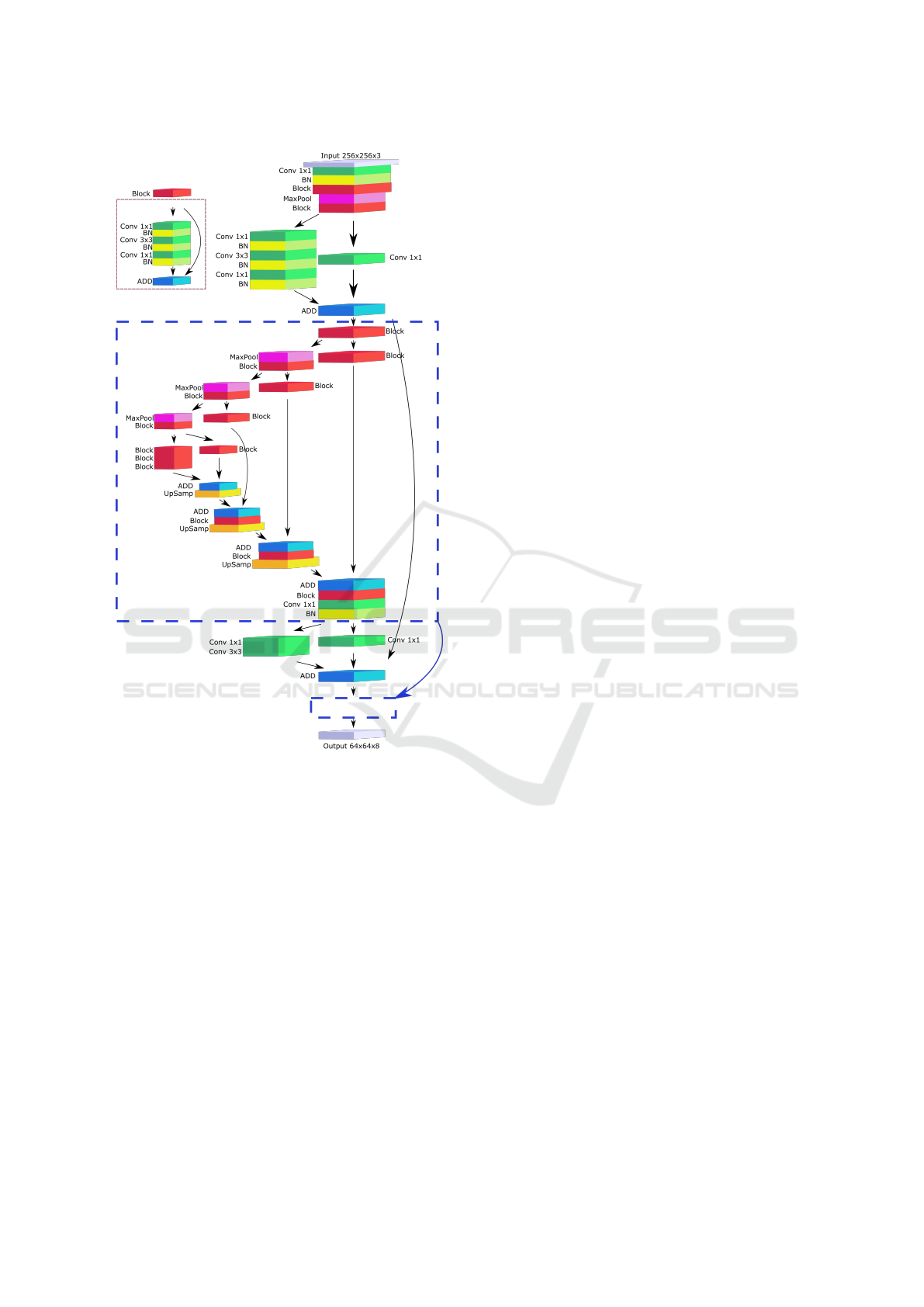
Figure 1: Architecture of neural network for detection of
object keypoints.
is similar to a basic block except that instead of di-
rect connection a 1 × 1 convolution is utilized in or-
der to calculate the residual. The feature map that is
fed to mentioned above residual block is determined
by a block consisting of 1× 1 convolution, batch nor-
malization, basic residual block, max pooling, and
the basic residual block. The first hourglass block is
followed by a residual block with 1 × 1 convolution
followed by 3 × 3 convolution in the first branch and
1 × 1 convolution in the second one.
The feature maps determined by both hourglass
blocks are utilized in calculating the loss. The mean
squared error has been used in the loss function
comparing the predicted heatmaps to a ground-truth
heatmaps with 2D gaussians centered at the object
keypoints. The neural network detects eight fiducial
keypoints that are represented by heatmaps on sepa-
rate output maps. The variance of 2D gaussians rep-
resenting locations of fiducial points in the images
from the training subset has been set to five pixels.
The neural network has been trained using RMSprop
optimizer with learning rate set to 1e-6. It has been
trained in 400 epochs and batch size set to 32.
2.3 Algorithm for 6D Object Pose
Tracking
The algorithm operates on sequences of RGB images
that are acquired by a calibrated camera. For ev-
ery object of interest a 3D sparse object model has
been prepared in advance. Every 3D model con-
sists of eight 3D locations that correspond to fidu-
cial keypoins of the object and which are detected
by the neural network. On every image, eight fidu-
cial objects points are determined using the hourglass
neural network, which has been discussed in Subsec-
tion 2.2. The positions of fiducial points on the ob-
jects were selected manually. Given the ground-truth
data the 3D positions of the fiducial points have been
determined afterwards. Using the parameters of the
calibrated camera they were then projected onto the
image plane. Every keypoint has been represented
by zero-mean normal distribution of pixel intensities,
centered on it and stored in a separate image. The ob-
ject keypoints have been stored in multidimensional
images with number of channels equal to number of
keypoints. Using the ground-truth data the 3D points
have been projected to image plane to determine a
window surrounding the object to cut the subimage
with object centered on it. The coordinates of sub-
windows were also used to cut subimages from the
multidimensional image, which were then resized to
64 × 64, see also output shape on Fig. 1.
During 3D object pose tracking, given the object
pose determined in the previous frame, a subimage
surrounding the object is determined and then scaled
to size of 256 × 256. Such an image is then fed
to hourglass neural network that determines the key-
points and represents them as heatmaps on separate
images of size 64 × 64. 2D locations of the keypoints
on such images are determined through seeking for
maximas in the heatmaps. The 2D locations of the
keypoints representing the object in current and the
previous frame were then fed to a Siamese neural
network (Majcher and Kwolek, 2021) to predict the
3D object pose, i.e. to calculate the 3D translation
and rotation of the object in the current frame. The
quaternion particle filter, which is outlined in Sub-
section 2.1, consisting of 200 particles has been em-
ployed to achieve 3D object pose tracking. A subset
of the particles without the particle with the small-
est weight is resampled and then each particle is pre-
Pose Guided Feature Learning for 3D Object Tracking on RGB Videos
577
dicted according to probabilistic motion model, dis-
cussed in Subsection 2.1. A priori probability distri-
bution determined in such a way is extended about
particle with pose determined by the Siamese neural
network. Given a particle state, the 3D keypoints are
projected onto the image. At keypoint coordinates,
the values of heatmaps are determined and then aver-
aged. Such averaged values have then been utilized
to calculate the values of particle weights. The likeli-
hood of the particle s can be expressed in the follow-
ing manner:
p(y|x = s) = e
−λ
d(s)−d
min
d
max
−d
min
2
(7)
where the mean distance d has been computed di-
rectly on the basis of the heatmap values: d(s) =
1.0−
1
N
∑
i
d
i
, where d
i
is a value given by the heatmap
map for the keypoint i projected onto the image plane,
whereas N is equal to eight and λ was determined ex-
perimentally.
3 EXPERIMENTAL RESULTS
At the beginning of this Section we discuss the eval-
uation metric for 6D pose estimation. Afterwards, we
present experimental results.
3.1 Evaluation Metric for 6D Pose
Estimation
We evaluated the quality of 6-DoF object pose esti-
mation using ADD score (Average Distance of Model
Points) (Hinterstoisser et al., 2013). ADD is defined
as average Euclidean distance between model vertices
transformed using the estimated pose and the ground
truth pose. It is defined as follows:
ADD = avg
x∈M
||(Rx + t) − (
ˆ
Rx +
ˆ
t)||
2
(8)
where M is a set of 3D object model points, t and R
are the translation and rotation of a ground truth trans-
formation, respectively, whereas
ˆ
t and
ˆ
R correspond
to those of the estimated transformation. This means
that it expresses the average distance between the 3D
points transformed using the estimated pose and those
obtained with the ground-truth one. The pose is con-
sidered to be correct if average distance e is less than
k
e
d, where d is the diameter (i.e., the largest distance
between vertices) of M and k
e
is a pre-defined thresh-
old (normally it is set to ten percent).
3.2 Evaluation of 3D Object Pose
Tracking
We evaluated our algorithm on a freely available OPT
benchmark dataset (Wu et al., 2017). It is a large 6-
DOF object pose tracking dataset that consists of 552
real-world image sequences. It includes RGB video
recordings of tracked objects, their 3D models, and
true poses. The dataset contains six models of vari-
ous geometric complexity. Object movement patterns
are diverse and the most natural scenario is FreeMo-
tion scenario in which the movements are in arbitrary
directions. As the OPT dataset does not contain the
object keypoints, we added eight keypoint locations
on each image from the FreeMotion scenario.
Table 1 presents root-mean-square errors (RMSE)
for 2D keypoints locations, which were obtained on
images from FreeMotion scenario of the OPT dataset.
It shows errors that were obtained for the four camera
views. In discussed table the RMSE errors achieved
by the hourglass neural network are compared with
the RMSE errors achieved by a simple neural net-
work. The simple neural network consisted of two
blocks with 32 and 64 3 × 3 2D convolutional fil-
ters, followed by 2 × 2 max pool and batch normal-
ization, which in turn were followed by three blocks
with 3 × 3 2D convolutional filters and batch normal-
ization, with 128, 256, and 512 filters each. On every
image a rectangle of size 128× 128 with the object in
its center has been cropped and then stored for evalu-
ation of the precision of determining the 2D locations
of the keypoints. As we can observe, the hourglass
architecture permits achieving considerably smaller
RMSE errors in comparison to errors achieved by the
simple network.
Table 1: RMSE achieved on the OPT dataset by our network
for fiducial keypoints estimation.
Left Right Back Front
Iron. (simple) 15.92 12.78 9.53 7.83
Iron. (hourglass) 2.26 2.70 0.65 0.66
House (simple) 10.92 11.59 14.57 16.60
House (hourglass) 4.24 3.22 3.35 2.05
Bike (simple) 15.45 14.69 6.68 9.42
Bike (hourglass) 2.14 2.39 0.93 2.74
Jet (simple) 10.40 14.70 16.39 19.50
Jet (hourglass) 2.32 1.10 4.78 8.85
Soda (simple) 10.63 8.77 19.35 2.61
Soda (hourglass) 4.91 0.65 5.06 1.83
Chest (simple) 18.42 21.67 17.26 14.80
Chest (hourglass) 9.06 10.83 3.80 4.84
Table 2 contains ADD scores that have been
achieved by our algorithm on the OPT benchmark
dataset in the FreeMotion scenario. All tracking
VISAPP 2022 - 17th International Conference on Computer Vision Theory and Applications
578
scores presented below are averages of three indepen-
dent runs of the algorithm with unlike initializations.
As we can observe, the average 10% ADDs are close
or better than 60%, except of the soda object, c.f. re-
sults in penultimate row in the discussed table.
Table 2: ADD scores [%] achieved on the OPT dataset by
our network, with PF-based object pose tracking.
ADD [%] Iron. House Bike Jet Soda Chest
beh., ADD 10% 81 80 62 81 35 25
beh., ADD 20% 99 99 90 95 43 29
left, ADD 10%
58 74 77 59 58 54
left, ADD 20% 93 95 96 81 93 89
right, ADD 10% 53 66 78 69 46 74
right, ADD 20% 84 89 98 78 96 96
front, ADD 10% 80 86 57 49 56 79
front, ADD 20% 99 100 89 77 84 96
Avg., ADD 10% 68 77 69 65 49 58
Avg., ADD 20% 94 96 93 83 79 78
The ADD scores presented in Tab. 3 have been
achieved by algorithm with a pose refinement. The
pose refinement has been realized by a Levenberg-
Marguardt (LM) algorithm. The pose represented by
the best particle has been used to initialize staring vec-
tor from which the LM optimization is run. Finally,
we combined the set of propagated particles with the
optimized particle, i.e. with pose determined in LM-
based object pose refinement. Comparing the ADD
scores achieved by the discussed algorithm against re-
sults presented in Tab. 2, we can observe that LM-
based pose refinement permits achieving better re-
sults. As we can see, for ADD 10% all ADD scores
are better, except for the ADD score achieved for the
soda object.
Table 3: ADD scores [%] achieved on the OPT dataset by
our network, with PF-based object pose tracking, and LM-
based pose refinement.
ADD [%] Iron. House Bike Jet Soda Chest
beh., ADD 10% 90 81 70 87 40 36
beh., ADD 20% 99 99 97 96 44 41
left, ADD 10% 68 74 82 64 59 60
left, ADD 20% 98 99 99 84 87 90
right, ADD 10% 64 71 89 76 32 70
right, ADD 20% 91 99 100 83 97 97
front, ADD 10% 81 86 59 65 63 83
front, ADD 20% 97 98 92 91 79 97
Avg., ADD 10% 72 78 75 73 49 62
Avg., ADD 20% 92 98 97 88 77 81
Table 4 compares results achieved by our algo-
rithm, where in the observation model the matching
was based on keypoints and heatmaps, and for com-
parison the observation model was based on object
segmentation and object rendering as in (Majcher and
Kwolek, 2021). As we can observe, none of the dis-
cussed algorithms obtains statistically better results.
However, it is worth noting that the observation model
based on keypoints and heatmaps is much simpler and
easier in implementation. Moreover, significant gains
in tracking speed are expected to be achieved due
to rapid progress in hardware dedicated to executing
neural networks as well as progress in compression of
models of the neural networks.
Table 5 contains AUC scores achieved by recent
methods in 6D pose tracking of six objects in the
FreeMotion scenario. As we can observe, our algo-
rithm attains better results than results achieved by
PWP3D, UDP, and ElasticFusion. In comparison to
results attained by algorithm (Tjaden et al., 2019), re-
sults achieved by our algorithm are also better. How-
ever, it is worth noting that the discussed results
are averages from all scenarios, including translation,
zoom, in-plane-rotation, out-of-plane rotation, flash-
ing light, moving light, i.e. scenarios in which the
errors are usually smaller than in the challenging free
motion scenario. Moreover, the discussed method de-
livers a single guess of each object’s pose, whereas
our algorithm outputs best poses together with prob-
ability distributions. The AUC scores by our algo-
rithm are noticeably better than results achieved in
(Majcher and Kwolek, 2021). Owing to using more
advanced neural network for object keypoints detec-
tion the whole algorithm for 6D object pose tracking
has been considerably simplified.
Figure 2 depicts ADD scores over time on se-
quences of images, which were achieved by our net-
work and PnP, and our network, PF and LM-based
object pose refinement. As we can observe, our algo-
rithm permits achieving far better tracking of the 6D
object pose on sequences of RGB images. The PnP
tend to lose object pose after some time in image se-
quences.
Table 6 presents running times that were achieved
on Jetson AGX Xavier board and a PC equipped with
Intel Core i5-10400F and GeForce RTX 2060. At the
moment, due to unoptimized implementation the run-
ning time is longer on the Jetson, but it is expected
that it will be shortened. The complete system for 6D
pose estimation has been implemented in Python lan-
guage with experiments performed using Keras.
4 CONCLUSIONS
In this work, we presented an algorithm for 3D ob-
ject pose tracking in RGB images. It employs pairs
of objects keypoints to predict rotation represented
by quaternion, as well as translation with the corre-
sponding delta translation. A single Siamese neural
network for a set of objects is trained on keypoints
from current and previous frame in order to predict
Pose Guided Feature Learning for 3D Object Tracking on RGB Videos
579
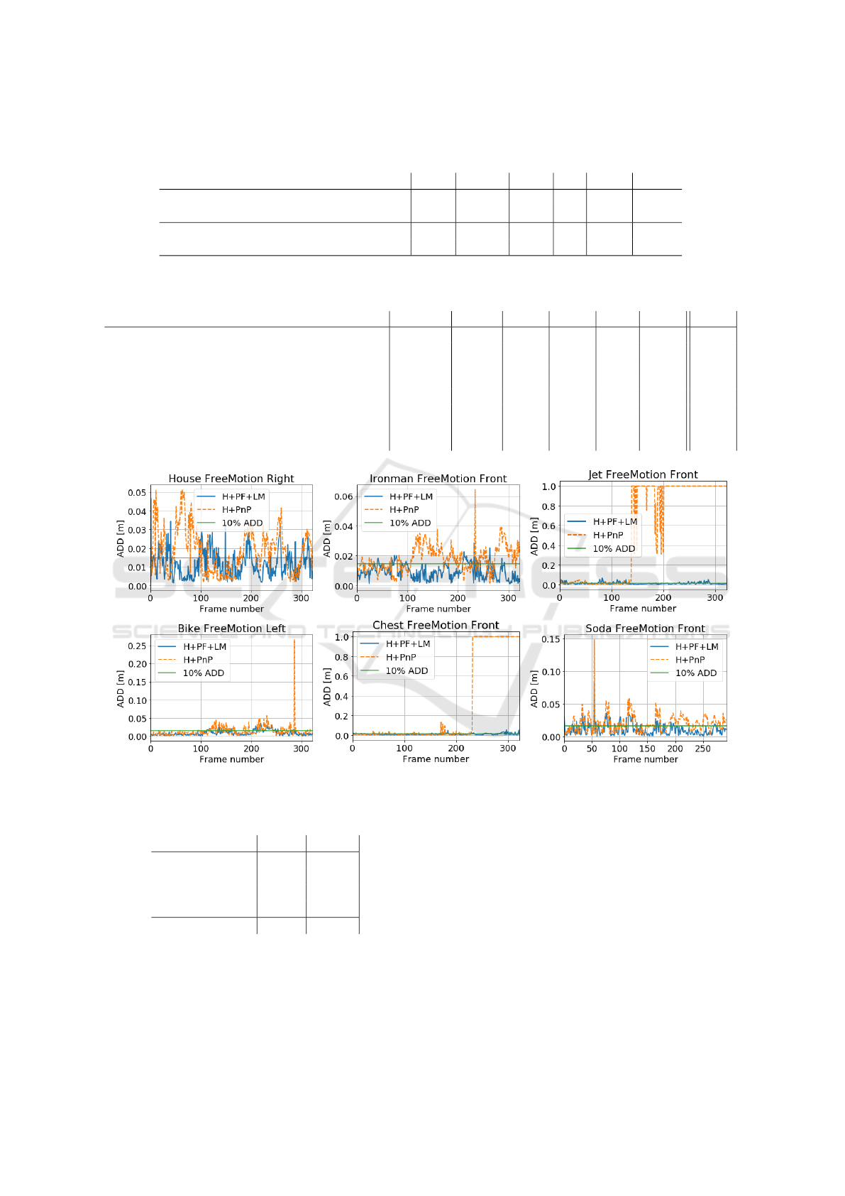
Table 4: ADD scores [%] achieved on the OPT dataset by our algorithm using keypoints and object rendering, as in (Majcher
and Kwolek, 2021).
Avg. ADD [%] Iron. House Bike Jet Soda Chest
object seg. and rend., 10% 71 67 67 66 49 58
object seg. and rend., 20% 93 79 91 85 74 85
keypoints and heatmaps (our), ADD 10% 72 78 75 73 49 62
keypoints and heatmaps (our), ADD 20% 92 98 97 88 77 81
Table 5: AUC scores achieved on OPT dataset in FreeMotion scenario (Wu et al., 2017), compared with AUC scores achieved
by recent methods.
Ironman House Bike Jet Soda Chest Avg.
PWP3D (all sc.) (Prisacariu and Reid, 2012) 3.92 3.58 5.36 5.81 5.87 5.55 5.02
UDP (all sc.) (Brachmann et al., 2016) 5.25 5.97 6.10 2.34 8.49 6.79 5.82
ElasticFusion (all sc.) (Whelan et al., 2016) 1.69 2.70 1.57 1.86 1.90 1.53 1.88
Reg. G-N. (all sc.) (Tjaden et al., 2019) 11.99 10.15 11.90 13.22 8.86 11.76 11.31
DQPP (FreeMotion) (Majcher and Kwolek, 2021) 10.32 13.27 11.88 10.33 8.90 7.60 10.38
Hourglass, LM (FreeMotion) 7.89 7.87 11.18 6.59 8.14 6.48 8.02
Hourglass, PF (w/o LM) (FreeMotion) 11.44 12.90 12.04 10.97 8.78 10.14 11.04
Our method (FreeMotion) 12.10 13.08 13.09 12.04 8.89 10.68 11.58
Figure 2: ADD scores over time on sequences of images, obtained by our network and PnP, and our network, PF and LM-based
pose refinement (plots best viewed in color).
Table 6: Running times [sec.].
PC Jetson
Hourglass 0.050 0.020
Siamese 0.030 0.007
PF 0.053 0.130
Other functions 0.017 0.023
Total 0.150 0.180
the 3D object pose. A keypoint-based pose hypoth-
esis is injected into the probability distribution that
is recursively updated in a Bayesian framework. We
demonstrated experimentally that keypoint locations
can be determined with sufficient precision by a single
hourglass neural network for a set of objects of inter-
est. The observation model of Bayesian filter has been
simplified without a noticeable drop in pose tracking
accuracy. In contrast to recent approaches, the al-
gorithm delivers the probability distribution of object
poses instead of a single object pose guess. LM-based
pose refinement permits achieving better results. The
algorithm runs in real-time both on a PC and a Jetson
AGX Xavier. In future work we are planning to in-
vestigate the performance of the algorithm in scenar-
ios with partial occlusions, including configurations
of the algorithm with and without object rendering,
VISAPP 2022 - 17th International Conference on Computer Vision Theory and Applications
580

taking into account the rendering capabilities of Jet-
son AGX Xavier.
ACKNOWLEDGEMENTS
This work was supported by Polish National
Science Center (NCN) under a research grant
2017/27/B/ST6/01743.
REFERENCES
Brachmann, E., Michel, F., Krull, A., Yang, M., Gumhold,
S., and Rother, C. (2016). Uncertainty-driven 6D pose
estimation of objects and scenes from a single RGB
image. In CVPR, pages 3364–3372.
Brachmann, E. and Rother, C. (2019). Neural-guided
RANSAC: Learning where to sample model hypothe-
ses. In IEEE/CVF Int. Conf. on Computer Vision
(ICCV), pages 4321–4330.
Chen, W., Jia, X., Chang, H. J., Duan, J., Shen, L., and
Leonardis, A. (2021). FS-Net: Fast shape-based net-
work for category-level 6D object pose estimation
with decoupled rotation mechanism. In IEEE Conf. on
Comp. Vision and Pattern Rec., CVPR, pages 1581–
1590. Comp. Vision Foundation / IEEE.
Egger, B., Sch
¨
onborn, S., Schneider, A., Kortylewski, A.,
Morel-Forster, A., Blumer, C., and Vetter, T. (2018).
Occlusion-aware 3D morphable models and an illumi-
nation prior for face image analysis. Int. J. Comput.
Vision, 126(12):1269–1287.
Fan, Z., Zhu, Y., He, Y., Sun, Q., Liu, H., and He, J.
(2021). Deep learning on monocular object pose
detection and tracking: A comprehensive overview.
arXiv 2105.14291.
Hinterstoisser, S., Lepetit, V., Ilic, S., Holzer, S., Bradski,
G., Konolige, K., and Navab, N. (2013). Model based
training, detection and pose estimation of texture-less
3D objects in heavily cluttered scenes. In Computer
Vision – ACCV 2012, pages 548–562. Springer.
Hu, Y., Hugonot, J., Fua, P., and Salzmann, M. (2019).
Segmentation-driven 6D object pose estimation. In
IEEE Conf. on Computer Vision and Pattern Rec.,
CVPR, pages 3385–3394.
Kaskman, R., Zakharov, S., Shugurov, I., and Ilic, S.
(2019). HomebrewedDB: RGB-D dataset for 6D pose
estimation of 3D objects. In IEEE Int. Conf. on Com-
puter Vision Workshop (ICCVW), pages 2767–2776.
Kehl, W., Manhardt, F., Tombari, F., Ilic, S., and Navab, N.
(2017). SSD-6D: Making RGB-Based 3D Detection
and 6D Pose Estimation Great Again. In IEEE Int.
Conf. on Computer Vision, pages 1530–1538.
Kutschireiter, A., Surace, C., Sprekeler, H., and Pfister, J.-P.
(2017). Nonlinear Bayesian filtering and learning: A
neuronal dynamics for perception. Scientific Reports,
7(1).
Majcher, M. and Kwolek, B. (2021). Deep quaternion pose
proposals for 6D object pose tracking. In Proceed-
ings of the IEEE/CVF Int. Conf. on Computer Vision
(ICCV) Workshops, pages 243–251.
Manhardt, F., Wang, G., Busam, B., Nickel, M., Meier, S.,
Minciullo, L., Ji, X., and Navab, N. (2020). CPS++:
Improving class-level 6D pose and shape estimation
from monocular images with self-supervised learning.
arXiv 2003.05848.
Newell, A., Yang, K., and Deng, J. (2016). Stacked hour-
glass networks for human pose estimation. In ECCV,
pages 483–499. Springer.
Pavlakos, G., Zhou, X., Chan, A., Derpanis, K. G., and
Daniilidis, K. (2017). 6-DoF object pose from seman-
tic keypoints. In IEEE Int. Conf. on Robotics and Au-
tomation (ICRA), pages 2011–2018.
Peng, S., Liu, Y., Huang, Q., Zhou, X., and Bao, H. (2019).
PVNet: Pixel-Wise Voting Network for 6DoF Pose
Estimation. In IEEE Conf. on Comp. Vision and Patt.
Rec., pages 4556–4565.
Prisacariu, V. A. and Reid, I. D. (2012). PWP3D: Real-
Time Segmentation and Tracking of 3D Objects. Int.
J. Comput. Vision, 98(3):335–354.
Rad, M. and Lepetit, V. (2017). BB8: A scalable, accurate,
robust to partial occlusion method for predicting the
3D poses of challenging objects without using depth.
In IEEE Int. Conf. on Comp. Vision, pages 3848–3856.
Tekin, B., Sinha, S. N., and Fua, P. (2018). Real-time
seamless single shot 6D object pose prediction. In
IEEE/CVF Conf. on Comp. Vision and Pattern Rec.
(CVPR), pages 292–301. IEEE Comp. Society.
Tjaden, H., Schwanecke, U., Sch
¨
omer, E., and Cremers, D.
(2019). A region-based Gauss-Newton approach to
real-time monocular multiple object tracking. IEEE
Trans. on PAMI, 41(8):1797–1812.
Tremblay, J., To, T., Sundaralingam, B., Xiang, Y., Fox, D.,
and Birchfield, S. (2018). Deep object pose estimation
for semantic robotic grasping of household objects. In
Proc. 2nd Conf. on Robot Learn., volume 87 of Proc.
of Machine Learning Research, pages 306–316.
Wang, Z., Li, W., Kao, Y., Zou, D., Wang, Q., Ahn, M., and
Hong, S. (2018). HCR-Net: A hybrid of classification
and regression network for object pose estimation. IJ-
CAI’18, pages 1014–1020. AAAI Press.
Whelan, T., Salas-Moreno, R. F., Glocker, B., Davison,
A. J., and Leutenegger, S. (2016). ElasticFusion. Int.
J. Rob. Res., 35(14):1697–1716.
Wu, P., Lee, Y., Tseng, H., Ho, H., Yang, M., and Chien,
S. (2017). A benchmark dataset for 6DoF object pose
tracking. In IEEE Int. Symp. on Mixed and Aug. Real-
ity, pages 186–191.
Xiang, Y., Schmidt, T., Narayanan, V., and Fox, D. (2018).
PoseCNN: A Convolutional Neural Network for 6D
Object Pose Estimation in Cluttered Scenes. In
IEEE/RSJ Int. Conf. on Intel. Robots and Systems.
Zakharov, S., Shugurov, I., and Ilic, S. (2019). DPOD: 6D
pose object detector and refiner. In IEEE/CVF Int.
Conf. on Computer Vision (ICCV), pages 1941–1950.
IEEE Computer Society.
Pose Guided Feature Learning for 3D Object Tracking on RGB Videos
581
