Comparing Monocular Camera Depth Estimation Models for Real-time

Applications

Abdelrahman Diab

, Mohamed Sabry

and Amr El Mougy

Computer Science Department, German University in Cairo, Cairo, Egypt

Keywords:

Depth Estimation, Monocular Camera, Computer Vision, Image Processing, Deep Neural Networks.

Abstract:

Monocular Depth Estimation (MDE) is a fundamental problem in the ﬁeld of Computer Vision with ongoing

developments. For the case of challenging applications such as autonomous driving, where highly accurate

results are required in real-time, traditional approaches fall short due to insufﬁcient information to understand

the scene geometry. Novel approaches utilizing deep neural networks show signiﬁcantly improved results, es-

pecially in autonomous driving applications. Nevertheless, there now exists a number of promising approaches

in literature and their performance has never been compared head-to-head. In this paper, a detailed evalua-

tion of the performance of four selected deep learning networks is presented. We identify a set of metrics to

benchmark the selected approaches from different aspects, especially those related to real-time applications.

We analyze the results and present insights into the performance levels of the various approaches.

1 INTRODUCTION

Nowadays, many production vehicles are equipped

with Advanced Driver Assistance Systems (ADAS)

that contain on board sensors such as cameras and

RADARs. This allows the integration of various mod-

ules for perception and scene understanding and ac-

cordingly contribute to higher safety standards. One

of the main modules to be integrated is depth estima-

tion, which can signiﬁcantly enhance the performance

of other modules such as Object classiﬁcation (Ciubo-

tariu et al., 2021) and Semantic Segmentation (Hoyer

et al., 2021). Depth estimation can be accurately

done using ranging sensors such as RADARs and Li-

DARs. However, these sensors are not widely inte-

grated in ADAS systems compared to cameras, es-

pecially monocular cameras. Depth estimation based

on cameras is possible, but is generally considered

a computationally-heavy task with less accurate re-

sults compared to ranging sensors. Accordingly, im-

proving the accuracy and reducing the complexity of

monocular depth estimation (MDE) would pave the

way for integrating it in more challenging applica-

tions that require high performance in real-time, such

as autonomous driving.

https://orcid.org/0000-0001-8375-7356

https://orcid.org/0000-0002-9721-6291

https://orcid.org/0000-0003-0250-0984

Traditional MDE approaches are based mainly on

computer vision (CV). These approaches are gener-

ally not computationally-heavy but do not produce

accurate results due to insufﬁcient scene geometry

for depth estimation. With modern advances in

GPUs, there has been increasing interest in using deep

neural networks for MDE (either solely or in con-

junction with CV ). These approaches produce rel-

atively more accurate results than CV alone but are

signiﬁcantly heavier, which means that their use in

real-time autonomous driving applications is ques-

tionable. Accordingly, the aim of this paper is to

compare the capabilities of the best performing net-

works across depth estimation benchmarks according

to their scores in accuracy metrics, inference speed,

qualitative results and their capability to perform in

real-time. The capabilities of the networks are tested

thoroughly on a vehicle in realistic settings, including

night-time driving, in order to gain deep insights into

their performance and behavior. To the best knowl-

edge of the authors, this is the ﬁrst paper to present

such an extensive performance analysis of MDE neu-

ral network models.

The remainder of this paper is structured follows:

In section 2 preliminary knowledge needed to under-

stand the work in this paper will be introduced, fol-

lowed by a review of previous works in the depth esti-

mation literature. In section 3 the four networks used

in the comparisons are introduced and their respec-

Diab, A., Sabry, M. and El Mougy, A.

Comparing Monocular Camera Depth Estimation Models for Real-time Applications.

DOI: 10.5220/0010883700003116

In Proceedings of the 14th International Conference on Agents and Artiﬁcial Intelligence (ICAART 2022) - Volume 3, pages 673-680

ISBN: 978-989-758-547-0; ISSN: 2184-433X

673

tive implementations are explained in detail. Follow-

ing this, the results of the work is shown in section 4

by comparing the networks across different aspects.

Finally, the paper is concluded in Section 5.

2 RELATED WORK

For the camera based depth estimation task, multiple

research directions were tackled such as the follow-

ing:

2.1 Handcrafted Feature-based

Methods

With the dawn of Artiﬁcial Intelligence (AI), sci-

entists began experimenting with machine learning

techniques to solve the Monocular Depth Estimation

(MDE) task. In a work that strongly inﬂuenced later

developments, (Saxena et al., 2005) used supervised

learning to predict the depth from monocular cues in

images, and used regression to estimate the pixel’s

depth value in an end-to-end manner. This work was

followed by many researchers proposing models to

estimate 3D structure from a 2d image using gradi-

ent sampling (Choi et al., 2015), perspective shift-

ing (Ladicky et al., 2014), analysis of light ﬂow (Fu-

rukawa et al., 2017), as well as many other approaches

(Hoiem et al., 2007; Konrad et al., 2013; Baig and

Torresani, 2016). These approaches were relatively

primitive with low performance results compared to

current deep learning approaches.

2.2 Deep Neural Networks based

Methods

Although there are many classical methods in the lit-

erature that tackle MDE, none of these techniques

produced sufﬁciently accurate results to provide a re-

alistic formula for solving the problem. This led to

scientists using deeper networks such as Convolu-

tional Neural Network (CNN)s to solve the MDE

problem. The models proposed used a variety of

learning methods, as well as many different variations

and conﬁgurations to produce their results.

2.2.1 Supervised Learning Models

This approach utilizes noisy and sparse reference

depth maps as ground truth labels to train super-

vised deep networks. These depth maps were con-

structed using point clouds from Light Detection And

Ranging (LIDAR) sensors or RGBD-cameras. (Go-

dard et al., 2017) proposed a CNN network archi-

tecture that was composed of two stacks. One of the

stacks focused on estimating the scene depth from a

global perspective, while the second stack performed

local reﬁnements to counter the global bias of the

ﬁrst stack. Along with this network architecture, the

authors also presented a new loss function that has

seen great use since its introduction. This new loss

function was named the Scale-Invariant loss function

(SILog). Instead of focusing on the general scale, this

function highlights the depth relation between the im-

age pixels.

Other papers such as (Lee et al., 2019) use a CNN-

based encoder network architecture to extract features

from the image. The extracted features are then input

to the decoder stage of the auto-encoder, which uses

the novel Local Planar Guidance (LPG) layer intro-

duced in their work in order to get the ﬁnal depth pre-

diction. In (Song et al., 2021) the LapDepth network

was introduced which uses a similar auto-encoder net-

work architecture to the network in (Lee et al., 2019)

but with Laplacian pyramid residuals in the decoder

stage to compute depth.

(Ranftl et al., 2021) introduced the DPT network

which uses a vision Transformer as the backbone for

feature extraction which can achieve better accuracy

than cnn networks but requires a larger dataset com-

pared to the encoder based networks.

Another work can be seen in (Bhat et al., 2020)

which is built around combining the advantages of

both CNNs and Vision Transformer (Vi-T)s. The

authors use a CNN feature extractor as their encoder,

combined with a simple upsampling decoder whose

output is connected to the Adabins mini-ViT module.

2.2.2 Self-supervised Learning Models

Supervised methods demand a large amount of

ground truth data, which require careful handpick-

ing and signiﬁcant time to produce. With this in

mind, efforts began to develop models that used self-

supervised learning for training models. These mod-

els trained networks to perform MDE using image

pairs from stereo camera setups (Garg et al., 2016;

Godard et al., 2017; Pillai et al., 2018) or synchro-

nized sequences of frames (Zhou et al., 2017).

Training with Stereo Images: (Garg et al., 2016)

proposed a CNN that retrieves depth maps by using

a stereo pair as input. The authors of this work intro-

duced a loss function that is equivalent to the photo-

metric difference between images. The model learns

the transformations necessary to recover depth infor-

mation using that loss function.

ICAART 2022 - 14th International Conference on Agents and Artiﬁcial Intelligence

674

Training with Monocular Video: (Zhou et al., 2017)

started research into this ﬁeld with their proposed

self-supervised model which estimates the camera

pose as well as the depth. (Yang et al., 2017) then

introduced a regularization method called 3D as-

smooth-as-possible to acquired depth maps and sur-

face normals from images. A previous work by (Yang

et al., 2018) exploited edge recognition to predict

depth and surface normals.

(Yin and Shi, 2018) introduced a network that

uses a geometric consistency loss function which ig-

nores occlusions and outliers to predict depth and

camera pose, and aided in performing optical ﬂow.

(Casser et al., 2018) made use of segmentation masks

to model dynamic objects, which was then used to

infer depth and visual odometry. At the same time,

(Mahjourian et al., 2018) developed a method to es-

timate ego-motion and depth simultaneously using a

geometric loss function that exploits temporal fea-

tures in the input. The term ego-motion refers to the

movement of the camera used in capturing between

different frames.

3 NETWORK

IMPLEMENTATIONS

The aim is to compare the performance of top monoc-

ular depth estimation networks to work under real-

time conditions. In this work, the four highest ranked

networks on the KITTI (Eigen split) benchmark are

compared. These networks are:

1. The AdaBins network in (Bhat et al., 2020).

2. The LapDepth network in (Song et al., 2021).

3. The Dense Prediction Transformer (DPT) net-

work in (Ranftl et al., 2021).

4. The Big to Small (BTS) network in (Lee et al.,

2019).

The following part will mention the details of the

four methods compared in this work starting with the

Big To Small network(BTS) (Lee et al., 2019), which

is ranked 4th on the KITTI (Eigen Split) Benchmark.

In their network implementation, they used an en-

coder network to extract features from the image,

which are then used as input to the decoder network.

The authors proposed the novel LPG layer in their

decoder, which performs the entire decoding process

with only 0.1M parameters.

The second model in this work’s comparison is

the LapDepth(Song et al., 2021) network which uses

a similar auto-encoder network architecture to BTS

with the exception of the decoder stage. In this stage,

they propose the use of Laplacian pyramid residuals

to compute depth. The estimated size of parameters

in the LapDepth decoder is 15M, which is nearly 150

times the features in the BTS decoder. LapDepth as

of the time of writing, is currently ranked second on

the KITTI depth estimation benchmark.

The third encoder-based network Adabins (Bhat

et al., 2020) is built around combining the advantages

of both CNNs and Vi-Ts. The authors achieve the

current state-of-the-art by using a CNN feature ex-

tractor as their encoder, combined with a simple up-

sampling decoder whose output is connected to the

Adabins mini-ViT module. This work shows the

large potential of discretization based depth estima-

tion, as well as the potential of network architectures

that do not follow the normal encoder-decoder-output

pipeline.

Finally the DPT network (Ranftl et al., 2021)

which uses a vision transformer network as the back-

bone for feature extraction in contrast to the other

three networks which used CNNs. The output of

the depth maps from this network is expected to have

better predictions around object boundaries and re-

tain its accuracy with varying input resolutions. How-

ever, this network’s variations have a large number of

parameters (more than 110M), and thus might yield

slower inference times.

4 RESULTS AND DISCUSSION

To evaluate a depth estimation model’s performance,

(Eigen et al., 2014) proposed a commonly utilized

evaluation method, which uses the following ﬁve

evaluation indicators to test the model’s overall accu-

racy, Root Mean Square Error (RMSE), RMSE-log,

Absolute Relative difference (AbsRel), Squared Rel-

ative difference (SqRel) and the Accuracies. These

metrics are used to compare the models’ accuracy on

the KITTI(Eigen split) benchmark.

RMSE =

∑

i=1



− d

∗



(1)

RMSELog =

∑

i=1



log(d

) − log (d

∗

)



(2)

AbsRel =

∑

i=1



− d

∗



∗

(3)

SqRel =

∑

i=1



− d

∗



∗

(4)

Comparing Monocular Camera Depth Estimation Models for Real-time Applications

675

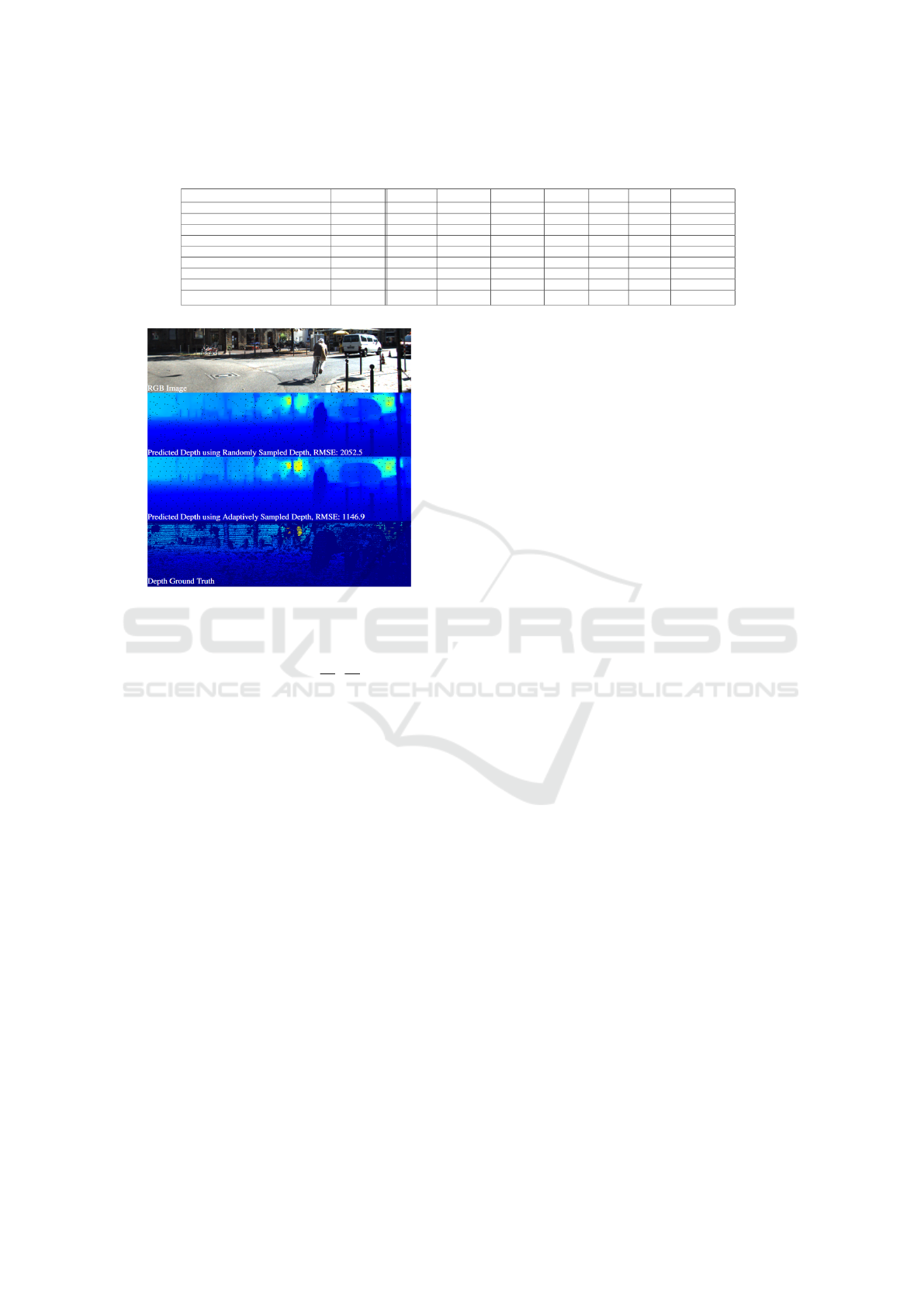
Table 1: Results of evaluating the different models on the KITTI (Eigen Split) Benchmark. The maximum depth is set to 80

for all networks. (↓) denotes a lower is better metric, while (↑) denotes a higher is better one.

Network No. Params δ < 1.25 ↑ δ < 1.25

↑ δ < 1.25

↑ AbsRel ↓ SqRel ↓ RMSE ↓ RMSE −log ↓

Adabins (Bhat et al., 2020) 78M 0.964 0.995 0.999 0.058 0.190 2.360 0.088

LapDepth(Song et al., 2021) 73M 0.962 0.994 0.999 0.059 0.212 2.446 0.091

DPT-Hybrid (Ranftl et al., 2021) 123.0M 0.959 0.995 0.999 0.062 0.226 2.573 0.092

BTS-ResNet-50 (Lee et al., 2019) 49.6M 0.954 0.992 0.998 0.061 0.250 2.803 0.098

BTS-ResNet-101 (Lee et al., 2019) 68.6M 0.954 0.992 0.998 0.061 0.261 2.834 0.099

BTS-ResNext-50 (Lee et al., 2019) 49.1M 0.954 0.993 0.998 0.061 0.245 2.774 0.098

BTS-ResNext-101 (Lee et al., 2019) 112.9M 0.956 0.993 0.998 0.059 0.241 2.756 0.096

BTS-DenseNet-121 (Lee et al., 2019) 21.3M 0.951 0.993 0.998 0.063 0.256 2.850 0.100

BTS-DenseNet-161 (Lee et al., 2019) 47.1M 0.955 0.993 0.998 0.060 0.249 2.798 0.096

Figure 1: A demonstration of a qualitative result from (Dai

et al., 2021) showing the result with a high RMSE and a low

RMSE.

Accuracies = % o f d

s.t. max(

∗

) = δ < thr

(5)

Where T denotes total number of pixels with

ground truth depth, d

∗

represents the ground truth

value of pixel i, and d

is the predicted depth of that

same pixel. Finally, thr signiﬁes the threshold, and is

usually set to 1.25, 1.25

, and 1.25

for evaluation.

Each of the functions mentioned above evalu-

ates the model in a different aspect than the others.

Equation 1 calculates the Root Mean Squared Error

(RMSE), which refers to the standard deviation of the

residuals. An example of the varying RMSE can be

seen in Fig. 1 as demonstrated in (Dai et al., 2021).

Similarly, the equation in 2 performs the standard

deviation, but the use of log makes it less affected

by large valued outliers which can explode the error

term to a very large number. Equation 3 of the ab-

solute relative error refers to the % of inaccuracy be-

tween the output and the input (×100 to get actual %).

Equation 4 is similar to equation 3, but the effect of

outliers is more exaggerated here. Equations 1, 2, 3,

and 4 are all lower-is-better metrics, which means

that a lower value for that metric indicates better re-

sults. Finally the equation in 5 refers to the % of

pixels that satisfy the threshold equation, and is used

to indicate the amount of pixels with small (δ < 1.25),

medium (δ < 1.25

), and large (δ < 1.25

) difference

from their ground truth values. Naturally, a higher-is-

better comparison is used for the accuracies metric.

4.1 KITTI(Eigen Split) Benchmark

Results

Table 1 lists the results of the models’ evaluation re-

sults on the KITTI (Eigen Split) benchmark (Geiger

et al., 2012), based on the ﬁve metrics mentioned in

the previous section. It is evident that the Adabins

(Bhat et al., 2020) network outperforms the other net-

works on all metrics across the board. However, this

alone does not qualify it to be the network of choice,

since accuracy is not the only value used to assess the

models.

It should also be noted that all of these net-

works were trained or ﬁne-tuned on the KITTI dataset

(Geiger et al., 2012) which they are being evaluated

on. Meaning that, in a live testing scenario, or while

testing on different data-sets (known as zero-shot

evaluation), the networks would likely score slightly

worse on the same evaluation metrics. The level of

accuracy degradation is proportional to how differ-

ent the input is from the KITTI dataset standard in

terms of input spatial resolution, lighting, scenery,

etc. The DPT-Hybrid (Ranftl et al., 2021) network

would likely suffer less degradation than the others

due to the following reasons:

The DPT (Ranftl et al., 2021) network was trained

on extra datasets other than the KITTI (Geiger et al.,

2012) dataset. This gives DPT an advantage when

performing evaluation on datasets it wasn’t trained on

(zero-shot evaluation), since it has seen a larger cor-

pus of data and is more generalized. This is especially

observable when comparing inﬁnite distance points

such as the sky. Networks trained on only the KITTI

dataset used a lidar pointcloud for their training, and

lidar can not capture inﬁnite distances. Consequently,

the network is confused as to what to predict for these

inﬁnity points and a seemingly random prediction is

given to the corresponding pixels.

An additional side-effect to the absence of labels

ICAART 2022 - 14th International Conference on Agents and Artiﬁcial Intelligence

676

Figure 2: A demonstration of the weight corrosion in the top

parts of the BTS and LapDepth networks. Which is due to

the absence of inﬁnite depth point labels for the sky during

training.

in the top part of the image (sky pixels), is that net-

works do not know how to train the weights respon-

sible for predicting pixels in that part. As a cause of

this, a visible ambiguous artifact is constantly shown

in the output near the top of the image. Both the BTS

(Lee et al., 2019) and Lap Depth (Song et al., 2021)

networks’ outputs suffer from this problem, and an

example of their weight corrosion is shown in Fig-

ure 2. On the other hand, DPT (Ranftl et al., 2021)

can handle these inﬁnite depth points and give a cor-

rect prediction for them most of the time.

4.2 Inference Speed

To have a robust system that can perform camera-

based depth estimation as well as obstacle avoid-

ance and Simultaneous Localization And Mapping

(SLAM), it needs to be able to assess the environment

and any minor changes in it in real-time. Addition-

ally, it is essential to do this on devices that are not

going increase the cost of hardware signiﬁcantly for

autonomous vehicle manufacturers.

To ensure these constraints are met, the nine

models’ performance were tested on the same hard-

ware. A PC with an i7-8800K, 32 GB of Memory

and 2 different GPU conﬁgurations. For a medium-

range Graphics Processing Unit (GPU), a Nvidia

GTX 1080Ti was used. For a higher-end GPU, the

Nvidia RTX 3090 was used. Their respective perfor-

mance results are shown in Tables 2, and 3.

To calculate this data the models ran over a series

of 849 frames, and calculate the frames per second

(fps) from that as (

849

total time taken

). Naturally, the time

of loading the models into the RAM and any other

processing time was not added to the timer, since it

is intended to run these models over large periods of

time on autonomous vehicles. Full resolution is de-

ﬁned to be the KITTI (Geiger et al., 2012) dataset’s

base resolution at 1216 × 352. Moreover, half reso-

lution is set to be 608 × 352, meaning that only the

width of the input is halved. This is because most

of the networks in this work’s comparison do not ac-

cept height values less than 352 as input. The Ab-

sRel metric value of each network was also included

to indicate their overall accuracy. Last but not least,

the number of trainable parameters (No. Params) for

each model is included since there is some correlation

between it and the inference speed.

It has been noticed that there is no direct corre-

lation between the type of network used and the fps

performance of the models. Instead, it is more likely

that the fps performance is reliant on the number of

parameters used by the network as well as its opti-

mization and the parallelization of its weights.

Finally, it is noted that the BTS (Lee et al., 2019)

network’s encoder variations seem to be dominant in

this competition, with the exception of BTS-ResNext-

101, which suffers from its large number of parame-

ters. The BTS-DenseNet-161 variation of the network

is praised with its great balance of accuracy and speed

nearing 10 fps on the medium range GPU at full res-

olution with only a 2% loss in overall accuracy from

the state-of-the-art.

4.3 Visual Comparison

In this section, qualitative analysis of the outputs of

the four networks is performed. Figure 3 shows exam-

ples of the network outputs, with the maximum depth

set to 80 meters for all networks.

It can be observed that all four networks perform

the given task very well, and that they are in fact able

to detect obstacles within the scene. The Adabins

(Bhat et al., 2020) network seems to be very conﬁdent

in its predictions. The LapDepth (Song et al., 2021)

network’s prediction is similarly good, but seems to

not have as conﬁdent predictions around smaller ob-

jects such as human heads and hands, as well as tree

boundaries.

The DPT (Ranftl et al., 2021) network on the other

hand has a solid output. This network’s output is

performs adequately around object boundaries, which

is due to the fact that the input data retains its size

throughout the entire network pipeline, and therefore

ﬁne-grained details are not lost. Additionally, the ex-

tra data it was trained on allows it to predict depth at

inﬁnite depth points better than the other networks.

The BTS (Lee et al., 2019) network has an output

that, while not ideal, is able to detect any obstacles in

view, and can do this at signiﬁcantly higher fps count

than all other networks. For the BTS network’s ex-

amples in Figure 3, the DenseNet-161 encoder based

variation was used, because it has a compromise be-

tween accuracy and speed, and it is recommended by

Comparing Monocular Camera Depth Estimation Models for Real-time Applications

677

Table 2: FPS comparison of all nine networks’ fps performances using a medium budget GPU (Nvidia GTX 1080Ti).

Network No. Params AbsRel fps (full resolution) fps (half resolution)

Adabins (Bhat et al., 2020) 78M 0.058 4.16 7.03

LapDepth(Song et al., 2021) 73M 0.059 3.75 6.04

DPT-Hybrid (Ranftl et al., 2021) 123.0M 0.062 2.96 5.56

BTS-ResNet-50 (Lee et al., 2019) 49.6M 0.061 12.54 18.40

BTS-ResNet-101 (Lee et al., 2019) 68.6M 0.061 10.90 15.46

BTS-ResNext-50 (Lee et al., 2019) 49.1M 0.061 7.93 13.75

BTS-ResNext-101 (Lee et al., 2019) 112.9M 0.059 2.26 4.66

BTS-DenseNet-121 (Lee et al., 2019) 21.3M 0.063 12.01 17.00

BTS-DenseNet-161 (Lee et al., 2019) 47.1M 0.060 9.46 14.08

Table 3: FPS comparison of all nine networks’ fps performances using a higher budget GPU (Nvidia RTX 3090).

Network No. Params AbsRel fps (full resolution) fps (half resolution)

Adabins (Bhat et al., 2020) 78M 0.058 9.28 12.69

LapDepth(Song et al., 2021) 73M 0.059 5.77 9.034

DPT-Hybrid (Ranftl et al., 2021) 123.0M 0.062 10.11 15.13

BTS-ResNet-50 (Lee et al., 2019) 49.6M 0.061 15.99 20.92

BTS-ResNet-101 (Lee et al., 2019) 68.6M 0.061 13.71 17.80

BTS-ResNext-50 (Lee et al., 2019) 49.1M 0.061 16.36 20.61

BTS-ResNext-101 (Lee et al., 2019) 112.9M 0.059 11.41 15.59

BTS-DenseNet-121 (Lee et al., 2019) 21.3M 0.063 15.02 18.37

BTS-DenseNet-161 (Lee et al., 2019) 47.1M 0.060 10.83 14.52

the authors of the BTS paper. The variance of the out-

puts from each other is very small overall, but is still

visible nonetheless.

4.4 Real Time Testing

4.4.1 Electing a Network

From the combined results of Sections 4.1, 4.2, and

4.3, it is concluded that the BTS network gives the

highest performance results in terms of speed, with a

slight compromise in accuracy compared to the oth-

ers, but a sufﬁciently comprehensible output none-

the-less in the case of this work. Therefore this net-

work is selected to be the one the framework will be

built around, and used in the real-time test-drive situ-

ation with the limitations that this challenge incurs.

The ﬂexibility of the BTS network when it comes

to choosing the encoder is also a great added fea-

ture to using this network. This allows easy switch-

ing between encoder networks, to be able to choose

whichever one is appropriate for the task at hand.

4.5 Framework Implementation

4.5.1 Overall Framework Description

To be able to test the mentioned depth estimation net-

works, a Logitech C922 camera was attached to the

Self-Driving Car Lab prototype. The frames are fed

to the BTS model, which is determined in Subsec-

tion 4.4.1 to be the best model for the real-time testing

in this work. A simple python framework was made

to handle the model loading for the chosen encoder

of choice (BTS comes with 6), as well as any resiz-

ing, cropping or data augmentation necessary. The

encoder weights are loaded from the pre-trained im-

plementations available on the original BTS online

repository (Lee et al., 2019). A simplistic graphic

user interface is implemented to show the depth es-

timation output, and the original image side-by-side

for comparison, in addition to a fps counter to show

the number of frames the model outputs every sec-

ond. Example outputs of this framework are shown in

Figure 4

4.5.2 Improving the Output

The results of changing the maximum depth attribute

were tested by setting the maximum depth to { 30,

50, 80 } then visually analysing the output. There

was no notable difference between the outputs while

testing. The main difference between them was in the

pixel intensity of nearby objects in the depth maps

produced by shorter ranged settings, which is caused

by normalizing the output depth on a tighter range.

The maximum depth was set to be 80 meters for all

tests, which is the default setting.

4.6 Night Time Tests

In order for depth estimation to operate in a robust

manner, they have to perform well under difﬁcult

weather conditions as well as poor lighting conditions

such as night time and shadows. Currently, these are

ICAART 2022 - 14th International Conference on Agents and Artiﬁcial Intelligence

678

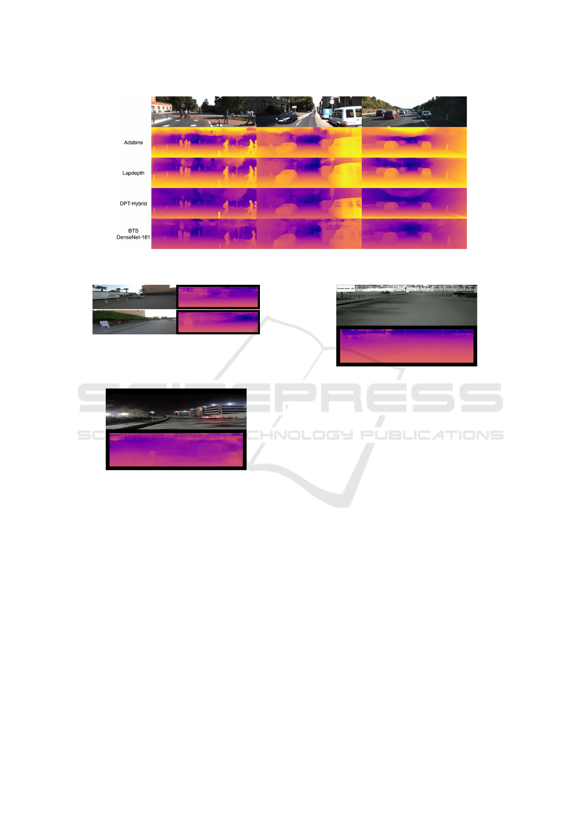
Figure 3: Comparison of the four contending networks on challenging images sampled from the KITTI (Geiger et al., 2012)

dataset’s validation set. The images are labelled according to the network used.

Figure 4: Real-time captured examples of the output of the

depth estimation framework proposed in this work while us-

ing the BTS-DenseNet-161 network option for predicting

the depth.

Figure 5: Prediction of depth estimation model using a nor-

mal HD monocular camera with no extra processing under

sufﬁcient lighting conditions at night time.

the largest challenges that face systems that are en-

tirely based on cameras. It has been found that the

network can still perform somewhat accurate predic-

tions when sufﬁcient lighting is found, and an exam-

ple of this is shown in Figure 5. However, in low illu-

mination conditions, the network’s output lacks useful

features that can correctly represent the scene.

To try and counter this problem, a HIKVISION 2

Megapixel Infra-Red Camera that would be tradition-

ally used for surveillance was utilised. This camera

would output an RGB colored image when sufﬁcient

lighting is present, then as soon as the lighting fades,

it automatically switches to Infrared mode. The out-

put of Infrared mode is a black and white image of the

same dimension as the RGB output.

The build framework was utilized for testing

again, but this time it was given the infrared camera

Figure 6: Top: input black and white image from infrared

camera. bottom: network prediction.

feed as input. The output of the network is quali-

tatively worse than the normal performance of day-

time testing. This is attributed to the network not be-

ing trained to handle the gray-scale images input to

it when the infrared mode is on, and therefore all the

predictions that relied on color information such as

color gradients are now lost. An example of the net-

work’s output with the Infrared mode on is shown in

Figure 6.

The results of the night vision approach seemed to

slightly improve the depth estimations results. How-

ever, there is room for improvement in this approach

which can yield a more robust night time perfor-

mance.

5 CONCLUSIONS

In this paper, the four highest bench-marked networks

on the KITTI (Eigen split) benchmark were explained

and their performance was compared quantitatively

and qualitatively. The BTS network was chosen as the

core of the real-time framework we implemented, as it

has the best compromise between speed and accuracy.

This framework was tested over several test-drives,

encompassing different lighting conditions. The ac-

curacy of the output is seemingly adequate for pro-

Comparing Monocular Camera Depth Estimation Models for Real-time Applications

679

ducing prototypes of practical applications.

Future work for monocular depth video applica-

tions could address problems like ﬂickering frames

and scale variance in a real-time manner. Addition-

ally, it would be interesting to add network function-

ality to predict inﬁnite distance points and mask out

the sky. Another approach to be investigated would

be to see if training a network for gray-scale image

depth prediction would lead to better results with the

infrared-mode output at night.

REFERENCES

Baig, M. H. and Torresani, L. (2016). Coupled depth learn-

ing. In 2016 IEEE Winter Conference on Applications

of Computer Vision (WACV), pages 1–10.

Bhat, S. F., Alhashim, I., and Wonka, P. (2020). Ad-

abins: Depth estimation using adaptive bins. CoRR,

abs/2011.14141.

Casser, V., Pirk, S., Mahjourian, R., and Angelova,

A. (2018). Depth prediction without the sensors:

Leveraging structure for unsupervised learning from

monocular videos.

Choi, S., Min, D., Ham, B., Kim, Y., Oh, C., and

Sohn, K. (2015). Depth analogy: Data-driven ap-

proach for single image depth estimation using gradi-

ent samples. IEEE Transactions on Image Processing,

24(12):5953–5966.

Ciubotariu, G., Tomescu, V.-I., and Czibula, G. (2021).

Enhancing the performance of image classiﬁcation

through features automatically learned from depth-

maps. In International Conference on Computer Vi-

sion Systems, pages 68–81. Springer.

Dai, Q., Li, F., Cossairt, O., and Katsaggelos, A. K. (2021).

Adaptive illumination based depth sensing using deep

learning. arXiv preprint arXiv:2103.12297.

Eigen, D., Puhrsch, C., and Fergus, R. (2014). Depth map

prediction from a single image using a multi-scale

deep network.

Furukawa, R., Sagawa, R., and Kawasaki, H. (2017). Depth

estimation using structured light ﬂow — analysis of

projected pattern ﬂow on an object’s surface. In 2017

IEEE International Conference on Computer Vision

(ICCV), pages 4650–4658.

Garg, R., BG, V. K., Carneiro, G., and Reid, I. (2016). Un-

supervised cnn for single view depth estimation: Ge-

ometry to the rescue.

Geiger, A., Lenz, P., and Urtasun, R. (2012). Are we ready

for autonomous driving? the kitti vision benchmark

suite. In 2012 IEEE Conference on Computer Vision

and Pattern Recognition, pages 3354–3361.

Godard, C., Aodha, O. M., and Brostow, G. J. (2017). Un-

supervised monocular depth estimation with left-right

consistency.

Hoiem, D., Efros, A. A., and Hebert, M. (2007). Recovering

surface layout from an image. International Journal

of Computer Vision, 75(1):151–172.

Hoyer, L., Dai, D., Chen, Y., Koring, A., Saha, S., and

Van Gool, L. (2021). Three ways to improve semantic

segmentation with self-supervised depth estimation.

In Proceedings of the IEEE/CVF Conference on Com-

puter Vision and Pattern Recognition, pages 11130–

11140.

Konrad, J., Wang, M., Ishwar, P., Wu, C., and Mukherjee,

D. (2013). Learning-based, automatic 2d-to-3d image

and video conversion. IEEE Transactions on Image

Processing, 22(9):3485–3496.

Ladicky, L., Shi, J., and Pollefeys, M. (2014). Pulling things

out of perspective. pages 89–96.

Lee, J. H., Han, M., Ko, D. W., and Suh, I. (2019). From big

to small: Multi-scale local planar guidance for monoc-

ular depth estimation. ArXiv, abs/1907.10326. Ac-

cessed: 2021-07-20.

Mahjourian, R., Wicke, M., and Angelova, A. (2018). Un-

supervised learning of depth and ego-motion from

monocular video using 3d geometric constraints.

Pillai, S., Ambrus, R., and Gaidon, A. (2018). Superdepth:

Self-supervised, super-resolved monocular depth esti-

mation.

Ranftl, R., Bochkovskiy, A., and Koltun, V. (2021). Vision

transformers for dense prediction. ArXiv preprint.

Saxena, A., Chung, S. H., and Ng, A. Y. (2005). Learning

depth from single monocular images. NIPS 18.

Song, M., Lim, S., and Kim, W. (2021). Monocular depth

estimation using laplacian pyramid-based depth resid-

uals. IEEE Transactions on Circuits and Systems for

Video Technology, pages 1–1.

Yang, Z., Wang, P., Wang, Y., Xu, W., and Nevatia, R.

(2018). Lego: Learning edge with geometry all at

once by watching videos.

Yang, Z., Wang, P., Xu, W., Zhao, L., and Nevatia, R.

(2017). Unsupervised learning of geometry with edge-

aware depth-normal consistency.

Yin, Z. and Shi, J. (2018). Geonet: Unsupervised learning

of dense depth, optical ﬂow and camera pose.

Zhou, T., Brown, M., Snavely, N., and Lowe, D. G. (2017).

Unsupervised learning of depth and ego-motion from

video.

ICAART 2022 - 14th International Conference on Agents and Artiﬁcial Intelligence

680