
Evaluating the Impact of Head Motion on Monocular Visual Odometry
with Synthetic Data
∗
Charles Hamesse
1,2
, Hiep Luong
2
and Rob Haelterman
1
1
Royal Military Academy, Department of Mathematics, XR Lab, Brussels, Belgium
2
Ghent University, imec - IPI - URC, Ghent, Belgium
Keywords:
Monocular Visual Odometry, Head Motion, Synthetic Data.
Abstract:
Monocular visual odometry is a core component of visual Simultaneous Localization and Mapping (SLAM).
Nowadays, headsets with a forward-pointing camera abound for a wide range of use cases such as extreme
sports, firefighting or military interventions. Many of these headsets do not feature additional sensors such as a
stereo camera or an IMU, thus evaluating the accuracy and robustness of monocular odometry remains critical.
In this paper, we develop a novel framework for procedural synthetic dataset generation and a dedicated motion
model for headset-mounted cameras. With our method, we study the performance of the leading classes of
monocular visual odometry algorithms, namely feature-based, direct and deep learning-based methods. Our
experiments lead to the following conclusions: i) the performance deterioration on headset-mounted camera
images is mostly caused by head rotations and not by translations caused by human walking style, ii) feature-
based methods are more robust to fast head rotations compared to direct and deep learning-based methods,
and iii) it is crucial to develop uncertainty metrics for deep learning-based odometry algorithms.
1 INTRODUCTION
The emergence of smart glasses or head-mounted ac-
tion cameras creates an entirely new set of challenges
and opportunities in the field of Simultaneous Local-
ization and Mapping (SLAM). In many applications
where such hardware is used, being able to estimate
3D information (ego-localization and scene geome-
try) would be beneficial. A core building block of
visual SLAM is visual odometry, which is the pro-
cess of estimating the camera position and rotation
changes between consecutive images. The monoc-
ular setup is of particular interest for these head-
mounted cameras, as they are naturally constrained
in size, weight and power. Monocular visual odom-
etry has the advantage of lower hardware costs and
less calibration efforts. Like most areas of com-
puter vision, monocular visual odometry has been
subject to a paradigm shift in favour of machine
learning methods. While often surpassing the perfor-
mance of traditional approaches in common bench-
marks (Yang et al., 2020), these methods come with
an increased computational complexity and in most
∗
The research presented in this paper is funded by the
Belgian Royal Higher Institute for Defense, in the frame-
work of the project DAP18/04.
cases, a decreased robustness. To this day, meth-
ods proposed in the literature are commonly eval-
uated on a handful of datasets, representing a spe-
cific use case and a specific sensor configuration,
such as KITTI (car) (Geiger et al., 2012) or Eu-
RoC (drone) (Burri et al., 2016). Unfortunately,
none of these common benchmarks represents im-
age sequences recorded with head-mounted cameras.
Therefore, a question arises: how to choose amongst
the monocular visual odometry classes for a head-
mounted camera system?
In light of the previous observations, we develop a
novel procedural synthetic dataset generator for head-
mounted camera sequences. We start by developing
a parametric headset motion model that allows us to
sample new headset trajectories. Then, we implement
a simulator framework using Unreal Engine (Epic
Games, 2020), which allows us to create synthetic
image sequences using the generated headset trajec-
tories. By putting the dataset generation in the exper-
iment loop, we effectively develop a novel methodol-
ogy for evaluating monocular visual odometry algo-
rithms, applied directly to study the impact of human
head motion. Our contributions are the following:
• A new headset motion model to simulate the mo-
tion of head-mounted cameras;
836
Hamesse, C., Luong, H. and Haelterman, R.
Evaluating the Impact of Head Motion on Monocular Visual Odometry with Synthetic Data.
DOI: 10.5220/0010881500003124
In Proceedings of the 17th International Joint Conference on Computer Vision, Imaging and Computer Graphics Theory and Applications (VISIGRAPP 2022) - Volume 5: VISAPP, pages
836-843
ISBN: 978-989-758-555-5; ISSN: 2184-4321
Copyright
c
2022 by SCITEPRESS – Science and Technology Publications, Lda. All rights reserved

• A novel simulation framework to create synthetic
image sequences in a variety of environments and
with arbitrary camera trajectories;
• New insights on the robustness of the monocular
visual odometry methods based on various exper-
iments using our framework.
2 RELATED WORK
We propose a review of the main classes of monocular
visual odometry, human head motion, and how 3D
engines are used for synthetic data generation to train
and test machine learning algorithms.
2.1 Monocular Visual Odometry
We propose to categorize the leading monocular vi-
sual odometry methods in four classes:
• Direct Methods. These methods optimize the di-
rect alignment of image regions in consecutive
frames. Minimizing a photometric error, these
methods directly operate on the intensity of the
pixels without requiring a feature extraction stage,
thus achieving relatively high frame rates. DSO
(Engel et al., 2018) is one such method and will
be used in our experiments.
• Feature-based Methods. A separate feature ex-
traction stage is used to create a set of image fea-
tures or keypoints to be matched in consecutive
frames. 3D camera poses and feature locations
are then estimated minimizing a geometric error.
The ORB-SLAM family (Mur-Artal and Tard
´
os,
2016) belongs to this class. We will use monoc-
ular ORB-SLAM3 in our experiments, disabling
its loop closure and global optimization features.
• Pure Deep Learning Methods. The first meth-
ods to use deep learning for visual odometry con-
sisted of large convolutional neural networks set
to take image pairs as input and return 6 DoF
pose changes (Agrawal et al., 2015; Zhou et al.,
2017; Godard et al., 2019). However, since ge-
ometry constraints or online optimization are not
used during evaluation in these “pure” deep learn-
ing methods (as inference consists in a single for-
ward pass of the network), their performance is
limited.
• Hybrid Methods. Combining deep neural net-
works with conventional, online optimization al-
gorithms, these methods enforce geometry con-
straints during inference. Convolutional neural
networks are used in the front-end for feature ex-
traction, single-view depth (Yang et al., 2020)
and/or two-view optical flow estimation (Zhan
et al., 2020). The back-end then uses classi-
cal nonlinear optimization algorithms. DeepV2D
(Teed and Deng, 2020) uses large hourglass
convolutional networks for feature extraction
then embeds a differentiable in-network Gauss-
Newton optimization layer. Since its codebase is
open-source and the method shows good general-
ization ability, we will use it in our experiments.
2.2 Head Motion
Let us start with noting the distinction between the
natural head motion (without headset) and headset
motion. Even though wearing a headset surely affects
the human head motion, the resulting motion will still
be primarily dictated by the human head movement.
In (Kristyanto et al., 2015), a kinematics analysis is
proposed to assess the extent and limitations of hu-
man head and neck movements. The proposed ranges
of movement for head rotations are 144 ± 20° for
yaw and 122 ± 20° for pitch and roll.
Recording head motion can be done using read-
ings from various sensors worn on the head (e.g.
IMUs) or motion analysis from video frames: in (Hi-
rasaki et al., 1999), video-based motion analysis is
used to capture the head motion of subjects walking
on a treadmill. (Jamil et al., 2019) uses a monoc-
ular camera placed in front of subjects walking and
running on a treadmill with a face detector to record
head motion and propose 2D trajectory models in the
frontal plane.
2.3 Synthetic Data Generation
With the strength of the whole gaming industry, 3D
engines keep improving significantly year after year.
The progress in photo-realism, their widespread avail-
ability and flexibility make that these engines are con-
sidered as serious alternatives to real-life measure-
ment campaigns to train and test machine learning
algorithms for computer vision tasks (Gaidon et al.,
2018). Arguably, Unreal Engine (Epic Games, 2020)
achieves the best photo-realism and is the most flexi-
ble, thus it is used in several simulators for computer
vision (Dosovitskiy et al., 2017; Shah et al., 2017;
Qiu et al., 2017). In addition to being able to simulate
scenarios that are expensive, time-consuming or dan-
gerous in real-life, synthetic data allows to arbitrarily
manipulate certain aspects in the scenes. Here, we
procedurally generate controlled variants of the same
dataset, isolating the effect of changing certain param-
eters related to headset motion.
Evaluating the Impact of Head Motion on Monocular Visual Odometry with Synthetic Data
837
3 HEADSET MOTION MODEL
We implement the translation and rotation compo-
nents separately: translation is based on real-life mea-
surements, described in Section 3.1, and rotation is
implemented with a random process, explained in
Section 3.2. The motivation is that the translation
of a walking human’s head over time relative to their
body trajectory is predominantly dictated by the per-
son’s physical characteristics and pace, but the rota-
tion is mainly context-dependent. Developing a rota-
tion model based on the environment, the current ac-
tion or cognitive state of the person would be overly
complex for the experiments in this work, so we re-
strict ourselves to a generic model.
3.1 Translation Model
We start with capturing the movement of a headset
worn by different persons walking or running at dif-
ferent speeds. Our population sample consists of 6
volunteers, 2 females and 4 males, with mean age
25.6 ± 5.5 years, all without any known injury or
disability
1
. We ask the volunteers to wear a Mi-
crosoft HoloLens 2 headset while walking or run-
ning on a treadmill. On the HoloLens 2, we run cus-
tom software that exports the 3D position returned by
the closed-source visual-inertial multi-camera SLAM
system of the headset at 60 Hz. Hardware features of
the headset relevant for its SLAM system are 4 wide-
angle visible light cameras and a 9-axis IMU. In ad-
dition, we place large calibration chessboards around
the treadmill to create an ideal environment for visual
tracking. The positions returned by the HoloLens 2
are used as reference in our work. Note that this setup
(ideal tracking features around the headset, visual-
inertial multi-camera system) is highly different from
our target setup (monocular camera in uncontrolled
environments).
With this setup, we rely on the hypothesis that
the headset motion recorded with our setup is sim-
ilar enough to that which would be recorded with
other head-mounted cameras. For each volunteer, we
record sequences of 3 minutes at each of the follow-
ing speeds on the treadmill: 2, 3, 4, 6, 8, 10, 12 km/h
and note whether they run or walk. The volunteers
are asked to move as if they were trying to reach the
point forward at the horizon. We have 6 volunteers ×
7 speeds, thus 42 sequences. Throughout the paper,
we use the axis system pictured in Figure 1.
1
Arguably, this is a small sample. Such measurements
are hard to collect given the ongoing COVID-19 pandemic
and related lockdown measures. However, increasing the
sample size would be valuable for future work.
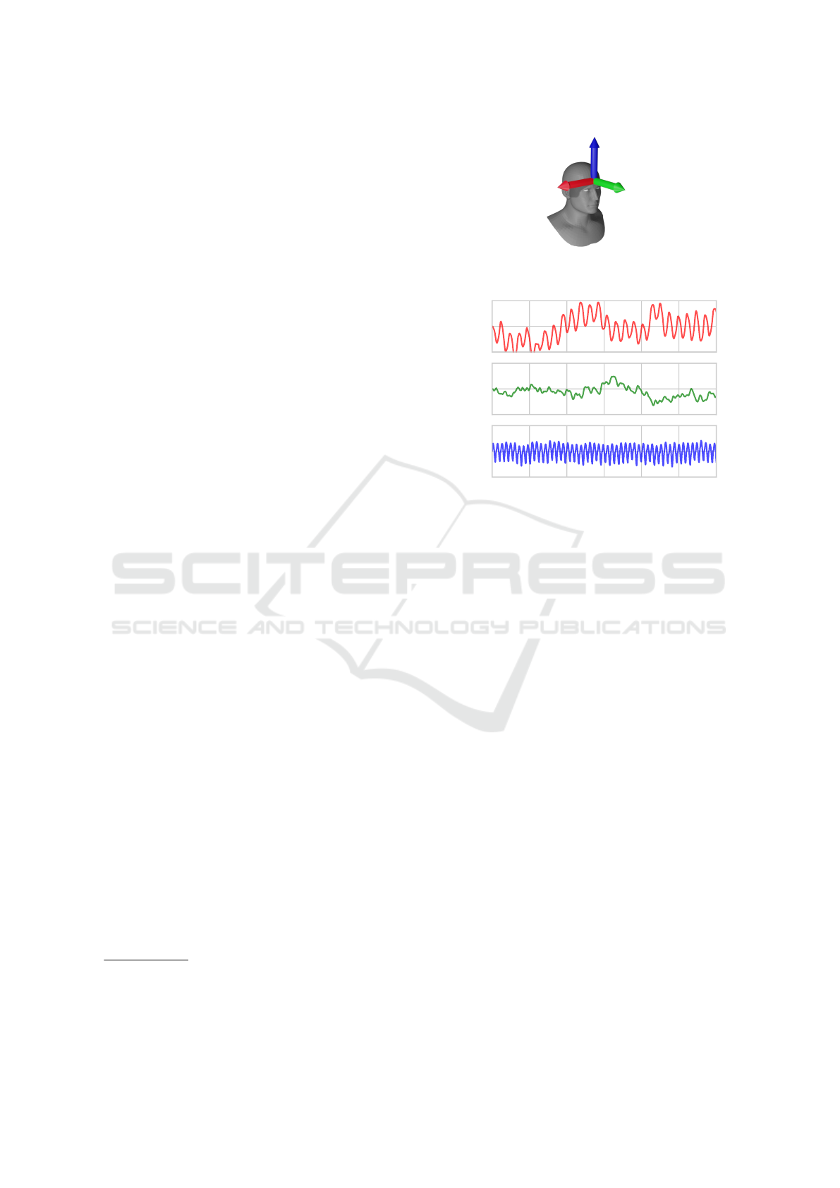
Figure 1: Coordinate system used throughout the paper. x
(red) is rightward, y (green) is forward and z (blue) is up.
−0.05
0.00
0.05
−0.05
0.00
0.05
0
5
10
15
20
25
30
−0.05
0.00
0.05
Time (s)
Position (m)
Figure 2: Extract of raw data from one subject walking on
the treadmill at 4 km/h. Headset position in x-y-z (resp.
red-green-blue, top to bottom). Here we show 30 seconds,
but whole sequences last 3 minutes.
We show an extract of raw data in Figure 2, where
we can clearly identify the periodic motion in the x-
axis (head balancing from side to side) and z-axis
(vertical bobbing). The bias of x and y signals vary
throughout the sequence because the subjects move
within the walkable area of the treadmill.
We now process the data to extract the headset
motion model. On each recorded sequence (i.e. 3
minutes of the same subject walking or running at the
same velocity), we apply these four steps:
1. We remove the bias to have the headset motion
relative only to the subject;
2. We split each sequence into strides (i.e. step cy-
cles starting and ending on the right foot);
3. We compute the template stride as a weighted av-
erage of all the available strides in each sequence;
4. We compute the noise distribution around each
template stride.
This will result in templates with noise distribu-
tions from which we can sample to generate new
headset trajectories.
3.1.1 Bias Removal
We isolate the headset motion from the moving sub-
ject inside the walkable area of the treadmill by sub-
VISAPP 2022 - 17th International Conference on Computer Vision Theory and Applications
838
tracting the average translation computed in a slid-
ing window. The window size should be roughly one
stride, so we use the period associated with the dom-
inant non-zero frequency of the Fourier transform of
the x signal (left-right component).
−0.05
0.00
0.05
−0.05
0.00
0.05
0
5
10
15
20
25
30
−0.05
0.00
0.05
Time (s)
Position (m)
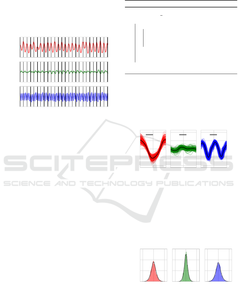
Figure 3: Head motion isolated by subtracting the moving
average and proposed stride splitting. Stride cuts are the
same in the three axes.
3.1.2 Stride Splitting
We set hand-made rules on the head motion signals
and their first and second time derivatives to deter-
mine the start of each stride. We use p
x
(i) to denote
the position in the x-axis at time i in a given sequence.
Since the sample rate is constant at 60 Hz, we com-
pute derivatives using the second-order centred differ-
ence approximation. A new stride is started if both of
these conditions are met:
• p
x
(i) > 0: the head is currently on the right;
• p
0
x
(i − 1) > 0 and p
0
x
(i + 1) < 0: the head is at the
rightmost position.
The resulting cuts are shown on Figure 3. We keep
the temporal scale consistent by linearly interpolating
each stride on 100 points and save the average time
needed to make a full stride.
3.1.3 Template Estimation
We compute a template (i.e. weighted average of all
strides) of each sequence using a robust M-estimator
as proposed in (Stewart, 1999). This is useful since it
handles the potential outliers that may appear in the
dataset, e.g. due to a volunteer making an odd step.
For each sequence, we gather all the stride signals
S
S
S
n
∈ R
3×L
with n = 1,...,N indexing all strides avail-
able in the sequence in three dimensions and L = 100
interpolated values. The goal of our stride average
estimator is to compute for each sequence a template
stride T
T
T ∈ R
3×L
.
Algorithm 1: Robust M-estimator.
input: S
S
S
n
n
n
for n = 1,...,N and h
k ← 0, T
T
T
0
=
1
N
∑
N
n=1
S
S
S
n
do
for n in 1, ...,N do
r = kT
T
T
k
− S
S
S
n
k
F
w
n
=
(
1 if r < h,
h/r otherwise.
end
k ← k + 1
T
T
T
k
= (
∑
N
n=1
w
n
S
S
S
n
)/(
∑
N
n=1
w
n
)
while kT
T
T
k
− T
T
T
k−1
k
F
> ε;
output: T
T
T
k
The robust estimator is described in Algorithm 1.
Through experimentation we find that the Huber pa-
rameter h that best separates the outliers from the in-
liers in our dataset is h = 0.1. On average, it takes
6 iterations until convergence, indicated by the tem-
plate varying by a quantity smaller than ε = 10
−7
in
consecutive iterations. The resulting stride template
for our example sequence is shown in Figure 4.
0
50
100
−0.04
−0.02
0.00
0.02
0.04
T
x
0
50
100
T
y
0
50
100
T
z
Stride progress (%)
Position (m)
Figure 4: All available strides in a sequence (line thickness
and opacity depending on the weight) and the resulting tem-
plate computed with the robust M-estimator in black.
3.1.4 Noise Analysis
For each sequence, we fit a generalized normal distri-
bution to the values around the template in each axis.
Generalized normal distributions add a shape parame-
ter β to the mean µ and variance σ, allowing to model
distributions where the tails are not Gaussian.
−0.02 0.00 0.02
0
50
100
150
β = 1.51
−0.02 0.00 0.02
β = 1.42
−0.02 0.00 0.02
β = 1.46
Density
Position (m)
Figure 5: Noise distribution (as a density) in each axis,
shown with the associated shape parameter β and the cor-
responding generalized normal distribution (black).
The β values found in our sequences (illustrated
in Figure 5) indicate that the distributions are between
Laplace and normal.
Evaluating the Impact of Head Motion on Monocular Visual Odometry with Synthetic Data
839
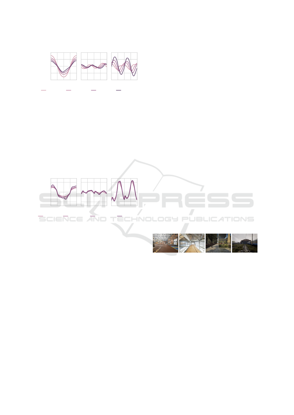
0
25 50 75
100
−0.050
−0.025
0.000
0.025
0.050
T
x
0
25 50 75
100
T
y
0
25 50 75
100
T
z
Position (m)
Stride progress (%)
2.0 km/h 3.0 km/h 4.0 km/h 6.0 km/h
Figure 6: Impact of increasing walking speed on the headset
motion of a single subject. Colour intensity increases with
speed.
To provide a larger overview of our dataset, we
propose additional visualizations aggregating differ-
ent templates. The impact of increasing locomotion
velocity is depicted in Figures 6 and 7. The former
shows how head motion changes when increasing the
walking speed from 2 to 6 km/h. We see that this
speed increase leads to a decrease of magnitude of
x motion (smaller left-right oscillations) and increase
of z motion (greater vertical bobbing, expected with
longer steps). All of our participants started jogging
0
25 50 75
100
−0.05
0.00
0.05
T
x
0
25 50 75
100
T
y
0
25 50 75
100
T
z
Position (m)
Stride progress (%)
8.0 km/h 10.0 km/h 12.0 km/h 14.0 km/h
Figure 7: Impact of increasing jogging speed on the headset
motion of a single subject. Colour intensity increases with
speed. For this particular subject we also have data at 14
km/h.
at the 8 km/h limit, which is why head motion fol-
lows a significantly different pattern at higher speeds.
In the next sections, we will use a multiplier param-
eter τ to modulate the amount of headset translation
that we desire to simulate when sampling new camera
trajectories.
3.2 Rotation Model
We propose a rotation model that allows to sample
random rotations and respects the range of movement
constraints described in (Kristyanto et al., 2015):
±72° for yaw and ±61° for both pitch and roll around
the forward looking direction. Parameterized by a ro-
tation rate parameter ρ in degrees, the procedure ex-
ecuted at each time step during the generation of tra-
jectories is as follows:
• Roll: we sample an angle from the uniform dis-
tribution U(−ρ, ρ), and add it to the roll angle of
the previous time step. If the resulting angle falls
outside of the boundaries (±61°), we set the angle
to the boundary value. The resulting roll rotation
is encoded using a quaternion q
r
.
• Pitch and yaw: we generate a new orientation with
rejection sampling. We start by sampling a ran-
dom vector uniformly on the unit sphere. To do
so, we sample a 3-vector from a normal distribu-
tion, then normalize it to lie on the unit sphere.
We reject it if it does not fall in the region delim-
ited by rotating the forward unit vector by ±72°
around the z-axis (yaw) and ±61° around the x-
axis (pitch). If it is rejected, we sample again.
If it is accepted, we make a partial rotation with
a fixed magnitude of ρ degrees towards this new
orientation. We do so using a spherical linear in-
terpolation between the pitch-yaw orientation at
the previous time step and the one just sampled.
The resulting pitch-yaw rotation is encoded using
a quaternion q
p,y
.
The complete rotation is then q = q
p,y
q
r
.
4 SYNTHETIC DATA
GENERATION
Our novel procedural synthetic dataset generator al-
lows the creation of sequences of images and camera
poses on the fly, in different maps and with arbitrary
camera trajectories. Our implementation is based on
(Qiu et al., 2017). We pick four Unreal Engine
(a) (b) (c) (d)
Figure 8: The four maps used in our framework: warehouse
(a), industrial office (b), modern city (c) and train yard (d).
maps with very different layouts representing indoor
and outdoor environments with various types of visual
features, shown in Figure 8. We export RGB frames
and ground truth camera poses at each time step of the
simulation. We model a camera with a 90° horizontal
field of view and 4/3 aspect ratio, producing images
with a resolution of 640x480 at 15 FPS.
5 EXPERIMENTS
Each of our experiments consists of two steps:
VISAPP 2022 - 17th International Conference on Computer Vision Theory and Applications
840

Figure 9: Images taken every 20 frames from the beginning of sequences in the modern city environment with translation
multiplier τ = 0 and rotation rate ρ = 3.
• Dataset generation: we sample a new trajectory
and generate sequences of images with headset
motion with various values for pace, translation
or rotation multiplier.
• Odometry evaluation: we run the different visual
odometry methods on the generated dataset and
evaluate their performance.
We compare DSO (Engel et al., 2018), ORB-
SLAM3 (Mur-Artal and Tard
´
os, 2016) and DeepV2D
(Teed and Deng, 2020). For DSO, we notice af-
ter some experimenting that the target point den-
sity needs to be decreased from 2000 to 500 for the
method to work best on our datasets. ORB-SLAM3
is used with default settings. DeepV2D is run with
weights trained on the NYU dataset (Burri et al.,
2016). Since we are interested in the performance of
visual odometry and not full-fledged SLAM, we dis-
able all loop closure or global optimization features in
ORB-SLAM3 and DeepV2D. Each algorithm is run
5 times on each sequence. We use relative pose er-
ror metrics between pairs of consecutive frames. For
i indexing the N frame pairs in the sequence, P
P
P
i,s
and
P
P
P
i,t
∈ SE(3) (special Euclidean group) denoting re-
spectively the source and target 4 × 4 pose matrices,
we have the following expressions for the discrep-
ancies D
D
D
i
∈ SE(3) and errors e
F
i
,e
R
i
and e
T
i
(respec-
tively full transformation, rotation only and transla-
tion only):
D
D
D
i
= (P
P
P
−1
i,s
P
P
P
i,t
)
−1
(
ˆ
P
P
P
−1
i,s
ˆ
P
P
P
i,t
) (1)
e
F
i
= kD
D
D
i
− I
I
I
4×4
k
F
(2)
e
R
i
= klog
SO(3)
D
D
D
R
i
k
2
(3)
e
T
i
= kD
D
D
T
i
k
2
(4)
where ˆ· denotes a quantity estimated by the odome-
try algorithm, D
D
D
T
i
∈ R
3
and D
D
D
R
i
∈ SO(3) (3D rotation
group) represent respectively the translation part and
the rotation part of the discrepancy matrix D
D
D
i
. The
logarithm log
SO(3)
is a map from SO(3) to so(3), the
Lie algebra of SO(3). In our evaluation, we use the
RMS of the errors over all N frame pairs.
5.1 Straight Baseline Trajectories
In each of the four maps shown in Figure 8, we define
a straight, walkable trajectory of 20 meters. On top
of each of these baseline trajectories, we sample from
our headset motion model using a template randomly
picked among our available templates with the usual
walking speed of 4 km/h. Since we model a camera
that records at 15 FPS, we have 270 images per se-
quence. We generate variants of the same sequence
with different values for the translation multiplier
τ = [0,1,2] and for the rotation rate ρ = [0,1,2,3].
Note that the translation multiplier only applies to the
headset motion, not the baseline trajectory. There-
fore, the synthetic dataset for this experiment consists
of 4 × 3 × 4 = 48 image sequences. Figure 9 shows
images taken from the synthesized sequences in the
modern city map and highlights the effect of the rota-
tion rate ρ set to 3 with straight trajectories (τ = 0).
Looking at the performance of DSO in Figure 10,
we notice that tracking gets lost in all four maps at a
certain rotation rate. That happens especially early in
the warehouse environment. In fact, this environment
features lots of small details (e.g. shelf corners) and
colours that do not stand out importantly in greyscale
(in which DSO works). This is contrasting with the
train yard environment, which has many large high-
gradient regions. Moreover, increasing the rotation
multiplier ρ steadily deteriorates the rotation error.
The performance of ORB-SLAM3, shown in Fig-
ure 10, shows more robustness as it does not lose
tracking in any sequence. Its performance slightly de-
teriorates when increasing the headset motion transla-
tion multiplier, and it remains very robust to rotations
overall. However, in the train yard sequences with
τ = 0 and 1, we see that the performance seriously de-
teriorates at the higher rotation rates. This is because
the rotation in these sequences have made the camera
progressively point towards a region where very few
good feature points are found, as illustrated in Fig-
ure 11. The rotation error behaves similarly to that of
DSO, except that it remains lower and tracking does
not get lost.
The performance of DeepV2D is shown in Fig-
ure 10. In translation-only trajectories (ρ = 0), the
errors are comparable to those of the traditional for-
mulations. Even though it does not lose tracking
when camera rotations start appearing, its perfor-
mance quickly deteriorates.
We now propose a comparison of the performance
of each pair of formulations:
Evaluating the Impact of Head Motion on Monocular Visual Odometry with Synthetic Data
841
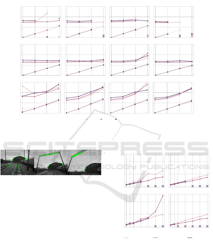
0
8
16
24
Industrial office Modern city Train yard Warehouse
0
2
4
6
e
T
RMS
e
R
RMS
0
8
16
24
0
2
4
6
e
T
RMS
e
R
RMS
0 1 2 3
0
8
16
24
0 1 2 3 0 1 2 3 0 1 2 3
0
2
4
6
e
T
RMS
e
R
RMS
τ = 0 τ = 1 τ = 2
Figure 10: Performance of DSO (top), ORB-SLAM3 (middle), DeepV2D (bottom) on the straight baseline experiment. The
horizontal axis represents the different values for the rotation rate ρ. The continuous lines represent the translation error e
T
RMS
and use the scale of the left vertical axis. The dotted lines represent the rotation error e
R
RMS
and use the scale of the right
vertical axis. The left and right vertical axes are shared across all four figures. A cross indicates that tracking was lost.
Figure 11: Sample images of a train yard sequence where
ORB features are becoming scarce.
DSO vs ORB-SLAM3. Although more complex due
to the feature extraction stage and therefore slower,
ORB-SLAM3 is much more robust to our sequences
with headset motion. Arguably, DSO could be helped
with a higher frame rate.
DSO vs DeepV2D. An important difference be-
tween the traditional formulations such as DSO and
DeepV2D is that DeepV2D will always return a pose,
it does not have a “tracking lost” state. This might
be a threat for some applications where position ac-
curacy is critical, highlighting the importance of esti-
mating the uncertainty of the predictions produced by
deep learning methods.
ORB-SLAM3 vs DeepV2D. In terms of perfor-
mance, both methods are affected similarly by trans-
lation, but ORB-SLAM3 remains more robust to ro-
tations. However, we notice that the relative per-
formance deterioration due to higher rotations in
the train yard sequences is greater in ORB-SLAM3
than in DeepV2D, indicating more robustness of
0
50
100
Industrial office Modern city
2 3 4
6
8 10 12
0
50
100
Train yard
2 3 4
6
8 10 12
Warehouse
e
F
RMS
Locomotion velocity (km/h)
DeepV2D ORB-SLAM3 DSO
Figure 12: Performance of DSO, ORB-SLAM3 and
DeepV2D on the locomotion speed experiment. A cross
indicates that tracking was lost. For simplicity, here we use
the full transformation error e
F
.
DeepV2D to a scarcity of good feature points.
5.2 Varying Locomotion Speed
We keep the same baseline trajectories as in the previ-
ous experiment but sample different headset motions:
VISAPP 2022 - 17th International Conference on Computer Vision Theory and Applications
842

we use the templates for all locomotion speeds avail-
able for a given subject, keep the head motion trans-
lation to the natural scale τ = 1 and rotation rate to
ρ = 2. The speeds used are 2, 3, 4, 6, 8, 10 and 12
km/h, in the same four maps.
We show the performances of DSO, ORB-
SLAM3 and DeepV2D in Figure 12. DSO lost track-
ing in many cases at higher speeds, which further
highlights its sensitivity to fast camera motion. Re-
call that all subjects started running (resulting in a
greater amplitude of headset motion) at the limit of
8 km/h, which is close to the average speed at which
DSO starts to fail in our sequences (7.5 km/h). The
performance of ORB-SLAM3 corresponds to previ-
ous observations: increased viewpoint changes lead
to a deterioration of the performance.
6 CONCLUSION
With our headset motion model and synthetic dataset
generator, we performed experiments on image se-
quences exhibiting various aspects of headset motion
parameterized to test the limits of monocular visual
odometry methods. Our three main findings are:
1. The main challenge for monocular visual odome-
try on headsets is rotation. Even slight rotations
can have important negative effects on the per-
formance of the three classes of algorithms that
we have studied. The head translation induced by
walking does not significantly deteriorate the per-
formance of monocular visual odometry.
2. Among the three methods that we have evalu-
ated, the feature-based ORB-SLAM3 is by far the
most robust. Deep learning-based methods such
as DeepV2D have a strong potential, for example
with their ability to estimate dense depth maps,
but it is critical to implement systems to ensure
that the properties of conventional features such as
invariance to translation or rotation, high localiza-
tion accuracy or robustness to image degradations
(noise, motion blur, etc.) are conserved.
3. Developing a robust measure of uncertainty for
the predicted poses is critical for deep learning-
based methods, since by default they will always
produce a prediction and not fall into a “tracking
lost” state, thereby failing silently.
REFERENCES
Agrawal, P., Carreira, J., and Malik, J. (2015). Learning to
see by moving. CoRR, abs/1505.01596.
Burri, M., Nikolic, J., Gohl, P., Schneider, T., Rehder, J.,
Omari, S., Achtelik, M. W., and Siegwart, R. (2016).
The euroc micro aerial vehicle datasets. The Interna-
tional Journal of Robotics Research.
Dosovitskiy, A., Ros, G., Codevilla, F., Lopez, A., and
Koltun, V. (2017). CARLA: An open urban driving
simulator. In Proceedings of the 1st Annual Confer-
ence on Robot Learning, pages 1–16.
Engel, J., Koltun, V., and Cremers, D. (2018). Direct sparse
odometry. IEEE Transactions on Pattern Analysis and
Machine Intelligence, 40:611–625.
Epic Games (2020). Unreal engine.
Gaidon, A., L
´
opez, A. M., and Perronnin, F. (2018). The
reasonable effectiveness of synthetic visual data. In-
ternational Journal of Computer Vision.
Geiger, A., Lenz, P., and Urtasun, R. (2012). Are we ready
for autonomous driving? the kitti vision benchmark
suite. In Conference on Computer Vision and Pattern
Recognition (CVPR).
Godard, C., Mac Aodha, O., Firman, M., and Brostow, G. J.
(2019). Digging into self-supervised monocular depth
prediction.
Hirasaki, E., Moore, S., Raphan, T., and Cohen, B. (1999).
Effects of walking velocity on vertical head and eye
movements during locomotion. Experimental brain
research, 127:117–30.
Jamil, Z., Gulraiz, A., Qureshi, W. S., and Lin, C. (2019).
Human head motion modeling using monocular cues
for interactive robotic applications. In 2019 Interna-
tional Conference on Robotics and Automation in In-
dustry (ICRAI), pages 1–5.
Kristyanto, B., Nugraha, B. B., Pamosoaji, A. K., and Nu-
groho, K. A. (2015). Head and neck movement: Simu-
lation and kinematics analysis. Procedia Manufactur-
ing, 4:359 – 372. Industrial Engineering and Service
Science 2015, IESS 2015.
Mur-Artal, R. and Tard
´
os, J. D. (2016). ORB-SLAM2: an
open-source SLAM system for monocular, stereo and
RGB-D cameras. CoRR, abs/1610.06475.
Qiu, W., Zhong, F., Zhang, Y., Qiao, S., Xiao, Z., Kim, T. S.,
Wang, Y., and Yuille, A. (2017). Unrealcv: Virtual
worlds for computer vision. ACM Multimedia Open
Source Software Competition.
Shah, S., Dey, D., Lovett, C., and Kapoor, A. (2017). Air-
sim: High-fidelity visual and physical simulation for
autonomous vehicles. In Field and Service Robotics.
Stewart, C. V. (1999). Robust parameter estimation in com-
puter vision. SIAM Rev., 41(3):513–537.
Teed, Z. and Deng, J. (2020). Deepv2d: Video to depth with
differentiable structure from motion. In International
Conference on Learning Representations (ICLR).
Yang, N., von Stumberg, L., Wang, R., and Cremers, D.
(2020). D3vo: Deep depth, deep pose and deep uncer-
tainty for monocular visual odometry. In IEEE CVPR.
Zhan, H., Weerasekera, C. S., Bian, J., and Reid, I. (2020).
Visual odometry revisited: What should be learnt?
2020 IEEE International Conference on Robotics and
Automation (ICRA), pages 4203–4210.
Zhou, T., Brown, M., Snavely, N., and Lowe, D. G. (2017).
Unsupervised learning of depth and ego-motion from
video. In CVPR.
Evaluating the Impact of Head Motion on Monocular Visual Odometry with Synthetic Data
843
