Transformation-Equivariant Representation Learning with
Barber-Agakov and InfoNCE Mutual Information Estimation
Marshal Arijona Sinaga, T. Basarrudin and Adila Alfa Krisnadhi
Faculty of Computer Science, University of Indonesia, Depok, Indonesia
Keywords:
Representation Learning, Transformation-Equivariant, Mutual Information Estimation, Barber-Agakov,
InfoNCE.
Abstract:
The success of deep learning on computer vision tasks is due to the convolution layer being equivariant to
the translation. Several works attempt to extend the notion of equivariance into more general transformations.
Autoencoding variational transformation (AVT) achieves state of art by approaching the problem from the
information theory perspective. The model involves the computation of mutual information, which leads to a
more general transformation-equivariant representation model. In this research, we investigate the alternatives
of AVT called variational transformation-equivariant (VTE). We utilize the Barber-Agakov and information
noise contrastive mutual information estimation to optimize VTE. Furthermore, we also propose a sequential
mechanism that involves a self-supervised learning model called predictive-transformation to train our VTE.
Results of experiments demonstrate that VTE outperforms AVT on image classification tasks.
1 INTRODUCTION
The success of convolutional neural networks (CNN)
in computer vision tasks is due to the equiv-
ariant property (Hinton et al., 2011; Cohen and
Welling, 2016). Specifically, the CNN extracts fea-
tures/representations that are equivariant to the trans-
lation. In general, transformation-equivariant guaran-
tees the obtained representation changes in the same
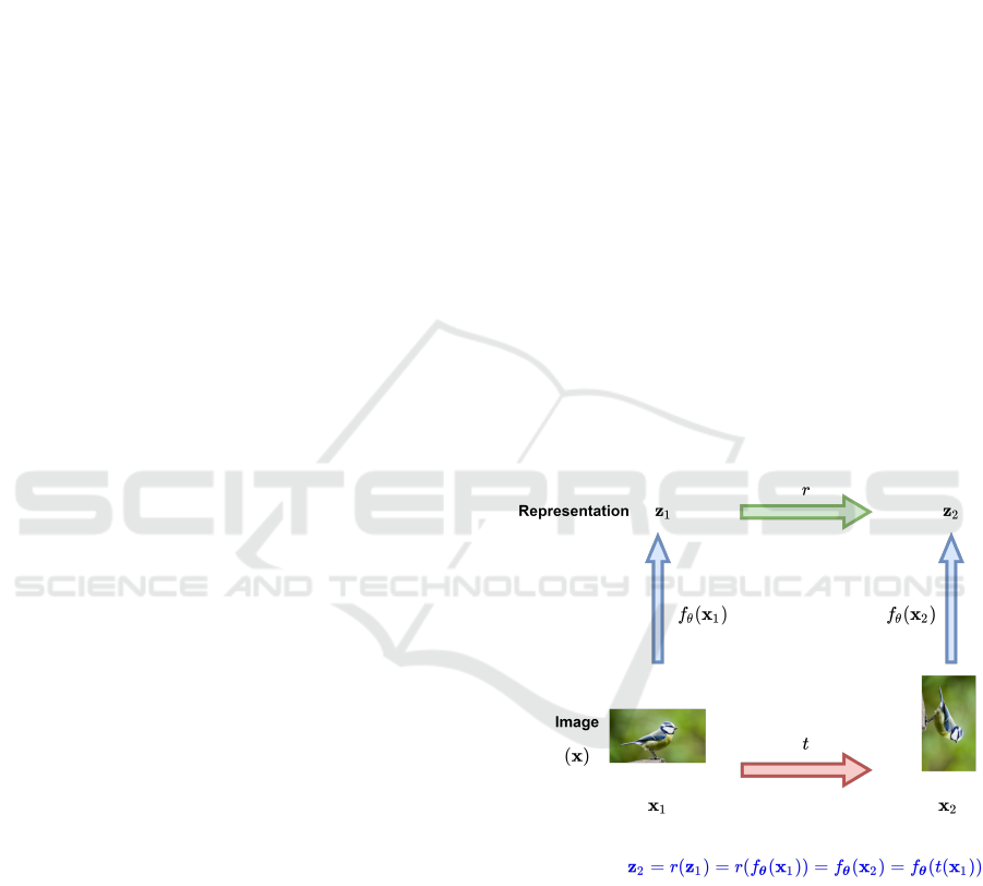
way as we transform the image. Figure 1 shows the
illustration of transformation-equivariant. This prop-
erty enables CNN to extract a better representation
structure from the given image. Some efforts have
been made such that CNN can handle various types
of transformations. However, current methods are
restricted to discrete transformations. Such circum-
stance limits the capacity of CNN to capture visual
structure under more complex transformation, includ-
ing continuous and non-linear transformations.
An unsupervised approach solves the limitation of
the transformations. State of the art utilizes an au-
toencoder called autoencoding transformation (AET)
(Zhang et al., 2019). This autoencoder reconstructs
the transformation t given the original image x and the
transformed image tx. The transformation t is drawn
from the affine and projective family of transforma-
tions. Another work extends the AET to an infor-
mation theory perspective, resulting in autoencoding
Figure 1: The illustration of transformation-equivariant.
The representation z
2
can be obtained in two ways. The first
approach is to feed a transformed image x
2
= t(x
1
) through
a function f
θ
, with t is the transformation in image space.
Another approach is to transform representation z
1
through
function r.
variational transformation (AVT) (Qi et al., 2019).
AVT adopts the notion of steerability and extends
it to an information theory perspective. The steerabil-
ity guarantees that we can transform the representa-
tion
ˆ
z the same way we transform the image x with-
Sinaga, M., Basarrudin, T. and Krisnadhi, A.
Transformation-Equivariant Representation Learning with Barber-Agakov and InfoNCE Mutual Information Estimation.
DOI: 10.5220/0010880400003122
In Proceedings of the 11th International Conference on Pattern Recognition Applications and Methods (ICPRAM 2022), pages 99-109
ISBN: 978-989-758-549-4; ISSN: 2184-4313
Copyright
c
2022 by SCITEPRESS – Science and Technology Publications, Lda. All rights reserved
99

out requiring x (Cohen and Welling, 2017). From an
information theory point of view, we can view the
steerability property as the MI between the represen-
tation of the original image
ˆ
z, the representation of
the transformed image z, and the transformation t (Qi,
2019). The goal of AVT is to maximize MI I(z;
ˆ
z, t).
However, computing the closed-form of MI is often
intractable, especially for high-dimensional data. In-
stead, AVT estimates the MI by decomposing the MI
into two terms and maximizing the lower bound of
one of them.
I(z;
ˆ
z, t) = I(
ˆ
z;z)+ I(z;t|
ˆ
z)
AVT maximizes I(z; t|
ˆ
z) by using Barber-Agakov es-
timation (Agakov, 2004). Results show that AVT
achieves promising results on image classification
tasks. However, It remains unclear whether term
I(
ˆ
z;z) gives the same performance as AVT.
This research investigates I(
ˆ
z;z) as an alterna-
tive objective to train an unsupervised transformation-
equivariant representation. Later on, we call the
alternative models as variational transformation-
equivariant (VTE). Our finding shows that maximiz-
ing I(
ˆ
z;z) without prior information is not feasible.
Instead, we train VTE into two stages. In the first
stage, we build a self-supervised learning model that
maximizes MI between transformation t and the rep-
resentation of the transformed image z. In the sec-
ond stage, we build VTE model and incorporate the
previous self-supervised learning model to maximize
I(
ˆ
z;z). Moreover, we apply Barber-Agakov (Agakov,
2004) and InfoNCE (van den Oord et al., 2018) MI es-
timation to maximize the MI, resulting in three differ-
ent models. Finally, we evaluate the proposed models
on image classification tasks. We conduct the classifi-
cation on two datasets: CIFAR-10 (Krizhevsky et al.,
2009) and STL-10 (Coates et al., 2011) datasets. The
main contributions of this paper are as follow:
• We design a mechanism to train VTE, an alterna-
tive version of AVT.
• We build a self-supervised model to help training
the VTE.
• We utilize Barber-Agakov and InfoNCE MI esti-
mation to train our VTE.
• We apply the proposed models as feature extractor
on image classification tasks.
We make our code available on Github.
1
The rest of this paper is organized as follows. In
Section 2, we cover works related to self-supervised
learning, transformation-equivariant representation,
and MI estimation methods. Section 3 gives a detailed
1
https://github.com/MarshalArijona/VTE
explanation of how to train VTE. In Section 4, we dis-
cuss the settings and results of experiments. Finally,
Section 5 gives the conclusion of this research.
2 RELATED WORKS
2.1 Transformation-Equivariant
Representation
The capsule net initiated the idea of general
transformation-equivariant representation (Hinton
et al., 2011; Wang and Liu, 2018). Capsule net takes
groups of neurons, which are responsible to capture
specific information of the image. Each capsule is
designed to be equivariant to specific transformations.
However, there was no rigorous algorithm to control
and guarantee the equivariance property for each
capsule.
Several works attempted to build a special con-
volution network that captures more types of trans-
formation operations. Group equivariant convolution
network (Cohen and Welling, 2016) introduces p4
and p4m groups to handle the equivariance for ro-
tation, translation, and reflection. This network pro-
duces a more complex visual structure which is bene-
ficial for the classification layer. Steerable CNN (Co-
hen and Welling, 2017) utilizes a filter bank that is
responsible to capture the equivariant property. An-
other work proposed dynamic routing for capsule net
(Lenssen et al., 2018) with concepts of equivariant
pose vectors and invariant agreements.
2.2 Self-supervised Learning
In general, self-supervised learning attempts to gen-
erate a surrogate label to enable supervised learning.
The surrogate label is synthesized from the part of
the data. (Noroozi and Favaro, 2016) divided the im-
age into several patches and permute the order of the
patches. Subsequently, they build a context-free net-
work to predict the index of the permutation. (Doer-
sch et al., 2015) also treat the images as grids/patches.
The idea is to predict the relative position of a ran-
dom grid given another grid that acts as the context.
(Noroozi et al., 2017) attempt to count the number of
features of the transformed images. In this research,
they restrict the transformation operation into scal-
ing and tiling. (Gidaris et al., 2018) apply discrete
rotation on the image and ask the model to predict
the type of rotation. (Dosovitskiy et al., 2016) apply
several transformations to the image. Subsequently,
they assign the same surrogate label to the original
ICPRAM 2022 - 11th International Conference on Pattern Recognition Applications and Methods
100

image and the transformed images. Finally, a classi-
fier is asked to predict the surrogate class. Most self-
supervised methods require some transformation op-
erations to train the model. However, the transforma-
tions are restricted to the pseudo label on which the
model is trying to solve. Furthermore, there is no ex-
plicit algorithm that guarantees the model preserves
the equivariant property.
2.3 Mutual Information Estimation
Given two random variables x and y, the mutual in-
formation I quantifies the amount of information (in
nat or bit) obtained about x after observing y or vice
versa. Mathematically, MI is defined by:
I(x; y) = E
p(x,y)
p(x, y)
p(x)p(y)
= E
p(x,y)
p(x|y)
p(x)
= E
p(x,y)
p(y|x)
p(y)
(1)
Computing MI is often intractable. Specifically, the
source of intractability is due to the unavailability to
the conditional distribution p(x|y). Furthermore, it
is often that we only have samples from the joint
distribution. Therefore, sample-based methods are
developed to estimate MI. In general, there are two
approaches to estimating MI: taking the variational
lower bound of MI and taking the variational upper
bound of MI.
Barber-Agakov MI estimation (Agakov, 2004) ap-
proximates the p(x|y) with a variational distribution
q(x|y) to obtain the lower bound of MI. This ap-
proach is relatively easy to compute but gives a high
bias. Another approaches transformed q(x|y) into an
unnormalized form by introducing a partition func-
tion Z (Nguyen et al., 2010; Donsker and Varadhan,
1975). However, those approaches require the sam-
ples from the marginal distribution, which we want to
avoid. InfoNCE (van den Oord et al., 2018) obtains
the lower bound by incorporating a contrastive loss
approach. The advantage of this method is the low
variance of the estimation. This method requires the
positive pair and the negative pairs of samples. How-
ever, the method is heavily dependent on the number
of samples.
We can adopt the Barber-Agakov method to ob-
tain the upper bound of MI. (Alemi et al., 2017) ap-
proximate the marginal distribution p(x) with a vari-
ational distribution q(x). However, approximating
the marginal distribution without prior information is
challenging, especially on high dimensional data. The
Leave-one-out (Poole et al., 2019) method attempts to
approximate p(x) by taking the sum of p(x
i
|y
j
) over
the samples (x
i
, y
j
), except y
i
. y
i
is the correspond-
ing pair of x
i
. Another approach incorporates a con-
trastive method to derive the variational upper bound
of MI (Cheng et al., 2020).
In this research, we perform MI maximization
with the help of Barber-Agakov and InfoNCE esti-
mation. Both methods only require samples from the
joint distribution, which fit the problem we aim to
solve.
3 VARIATIONAL
TRANSFORMATION-
EQUIVARIANT
3.1 The Generalization of
Transformation-Equivariant
Representation
Let
ˆ
z ∈ Z be the representation of image x ∈ X and
t : X × T → X be a transformation that involves im-
age x and a transformation operation t. We have
z ∈ Z be the representation of a transformed image
t(x, t) = tx. We can view the transformation t as a
matrix. Representations
ˆ
z, z, and transformation t sat-
isfy the transformation-equivariant property if there
exists a function r : Z × T → Z, such that
z = r(z, t) = τ(t)(
ˆ
z) (2)
where τ(t) denotes a function that enable t to be ap-
plied in Z. Note that the representation z is com-
pletely determined by t and
ˆ
z (no need access to x).
This notion is called steerability (Cohen and Welling,
2017; Qi, 2019), which enables computing z by ap-
plying an independent transformation τ(t) to
ˆ
z.
From the information theory perspective, we can
model the notion of steerability as the MI between z,
and (
ˆ
z, t) (Qi, 2019). Here the MI is parameterized
by θ. Therefore, the goal is to find θ that maximizes
I
θ
(z;
ˆ
z, t).
θ
∗
= max
θ
I
θ
(z;
ˆ
z, t) (3)
The form I
θ
(z;
ˆ
z, t) is not feasible to compute. To en-
able the training, we decompose I
θ
(z;
ˆ
z, t) into:
I
θ
(z;
ˆ
z, t) = E
p
θ
(z,
ˆ
z,t)
p
θ
(z,
ˆ
z, t)
p
θ
(z) p
θ
(
ˆ
z, t)
= E
p
θ
(z,
ˆ
z,t)
p
θ
(
ˆ
z)p
θ
(z|
ˆ
z)p
θ
(t|z,
ˆ
z)
p
θ
(z) p
θ
(t|
ˆ
z)p
θ
(
ˆ
z)
= E
p
θ
(z,
ˆ
z,t)
p
θ
(z|
ˆ
z
p
θ
(z)
+ E
p
θ
(z,
ˆ
z,t)
p
θ
(t|z,
ˆ
z)
p
θ
(t|
ˆ
z)
= I
θ
(z;
ˆ
z) + I
θ
(z;t|
ˆ
z) (4)
Transformation-Equivariant Representation Learning with Barber-Agakov and InfoNCE Mutual Information Estimation
101
AVT aims to maximize I
θ
(z;t|
ˆ
z) as the objective func-
tion. In this paper, we investigate the performance of
an transformation-equivariant repersentation model
by maximizing I
θ
(
ˆ
z;z). We name this model as vari-
ational transformation-equivariant (VTE). Both AVT
and VTE encounter the intractable computation of
MI. AVT needs to compute the intractable posterior
p
θ
(t|
ˆ
z, z), while VTE needs to compute intractable
posterior p
θ
(z|
ˆ
z). Therefore we need to estimate the
MI. AVT utilizes Barber-Agakov estimation to max-
imize the MI. In this research, we maximize MI by
using Barber-Agakov (Agakov, 2004) and InfoNCE
MI estimation (van den Oord et al., 2018).
3.2 Transformation as Inductive Bias
Our preliminary experiments showed that maximiz-
ing MI I
θ
(
ˆ
z;z) without prior results in the model fails
to learn. Specifically, the model will assign a trivial
posterior probability given any pair of (
ˆ
z, z). There-
fore, we need to explicitly involve the transformation
t to train VTE.
We propose sequential mechanism to train the
VTE. The training comprises two phases of training.
In the first phase, we model the distribution of z. Re-
call that z is the representation of the transformed im-
age. We involve the transformation t the train the
model. Specifically, we build a self-supervised learn-
ing model that maximizes the MI I
ˆ
θ
(z;t), parame-
terized by
ˆ
θ. We call this model as the predictive-
transformation. Note that this objective function is
similar to AVT (I
θ
(z;t|
ˆ
z)), except without
ˆ
z. Due to
the absence of
ˆ
z, the obtained representation is not
guaranteed to be equivariant anymore. We maximize
the MI by using Barber-Agakov lower bound MI esti-
mation. Barber-Agakov estimation introduces a vari-
ational distribution q
ˇ
φ
(t|z), parameterized by
ˇ
φ to ap-
proximate p
ˆ
θ
(t|z).
I
ˆ
θ
(t;z) = H(t) − H(t|z)
= H(t) + E
p
ˆ
θ
(t,z)
log p
ˆ
θ
(t|z)
= H(t) + E
p
ˆ
θ
(t,z)
logq
ˇ
φ
(t|z)
+ E
p(z)
KL(p
ˆ
θ
(t|z)k q
ˇ
φ
(t|z))
≥ H(t) + E
p
ˆ
θ
(t,z)
logq
ˇ
φ
(t|z) (5)
H(.) and KL(.k.) denote the entropy and the
Kullback-Leibler divergence between two distribu-
tions, respectively. Since H(t) does not depend on
ˆ
θ and
ˇ
φ, we simply maximize
max
ˆ
θ,
ˇ
φ
E
p
ˆ
θ(t,z)
logq
ˇ
φ
(t|z) (6)
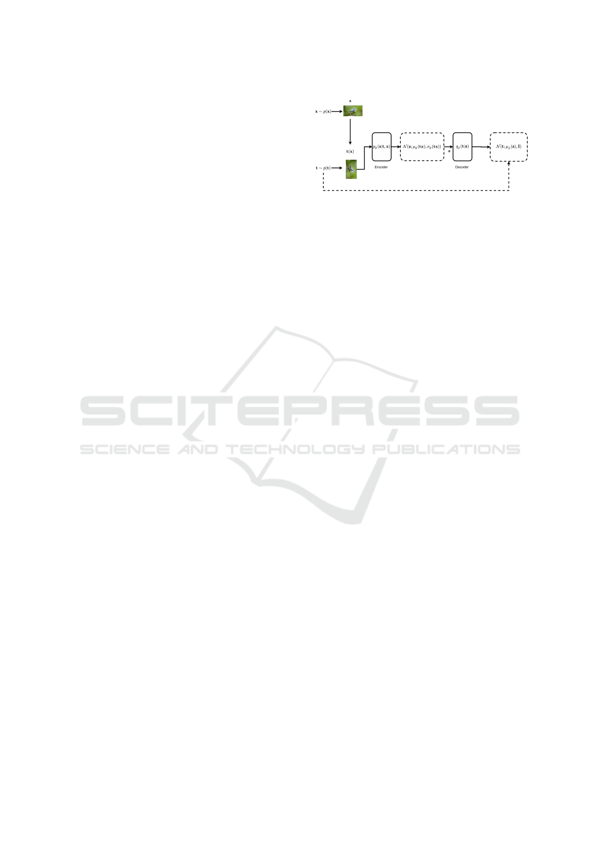
We implement the predictive-transformation in the
framework of autoencoder. Figure 2 shows the archi-
tecture of predictive-transformation.
Figure 2: The architecture of predictive-transformation
model. Transformed image is fed through the encoder p
ˆ
θ
.
The output of encoder is the mean µ
ˆ
θ
and the standard-
deviation σ
ˆ
θ
. The representation z is sampled and fed
through the decoder q
ˇ
φ
. The output of the decoder is the
mean µ
ˇ
φ
, which corresponds to the transformation t.
The encoder E
ˆ
θ
represents p
ˆ
θ
(z|tx). We assume that
p
ˆ
θ
(z|tx) is following a factored multivariate Gaussian
distribution N (z;µ
ˆ
θ
, σ
ˆ
θ
). Therefore, the output of the
encoder is the mean µ
ˆ
θ
and the standard-deviation σ
ˆ
θ
.
The decoder D
ˇ
φ
represents the variational distribution
q
ˇ
φ
(t|z). We also assume that q
ˇ
φ
(t|z) is a factored mul-
tivariate Gaussian distribution, with a constraint that
the standard-deviation sets to one: N (t;µ
ˇ
φ
, I). I de-
notes the identity matrix. Thus, the output of the de-
coder is the mean µ
ˇ
φ
.
For the second phase of training, we capture the
distribution of
ˆ
z by training the VTE network. The
goal is to maximize the MI I
θ
(
ˆ
z;z). We estimate
I
θ
(
ˆ
z;z) by using Barber-Agakov and InfoNCE esti-
mation. The optimization can be done through a
gradient-based method such as stochastic gradient de-
scent.
3.3 Barber-Agakov Lower Bound
Estimation
Following Equation 5, we derive the lower bound
of I
θ
(
ˆ
z;z) by introducing a variational distribu-
tion q
φ
(z|
ˆ
z), parameterized by φ to approximate
p
θ
(z|
ˆ
z). Furthermore, we incorporate the predictive-
transformation from the first phase of training to ob-
tain the representation z. We call this model as
VTEBArber-Agakov (VTEBA).
I
θ,
ˆ
θ
(
ˆ
z;z) = H(z) −H(z|
ˆ
z)
= H(z) + E
p
θ,
ˆ
θ
(t,
ˆ
z,z)
log p
θ,
ˆ
θ
(z|
ˆ
z)
= H(z) + E
p
θ,
ˆ
θ
(t,
ˆ
z,z)
logq
φ
(z|
ˆ
z)
+ E
p(
ˆ
z)
KL(p
θ,
ˆ
θ
(z|
ˆ
z)|| q
φ
(z|
ˆ
z))
≥ H(z) + E
p
θ,
ˆ
θ
(t,
ˆ
z,z)
logq
φ
(z|
ˆ
z) (7)
ICPRAM 2022 - 11th International Conference on Pattern Recognition Applications and Methods
102
In this phase, we do not optimize
ˆ
θ anymore. There-
fore, the objective function of VTEBA is maximizing
max
θ,φ
E
p
ˆ
θ,θ(t,
ˆ
z,z)
logq
φ
(z|
ˆ
z) (8)
Just like predictive-transformation, we treat
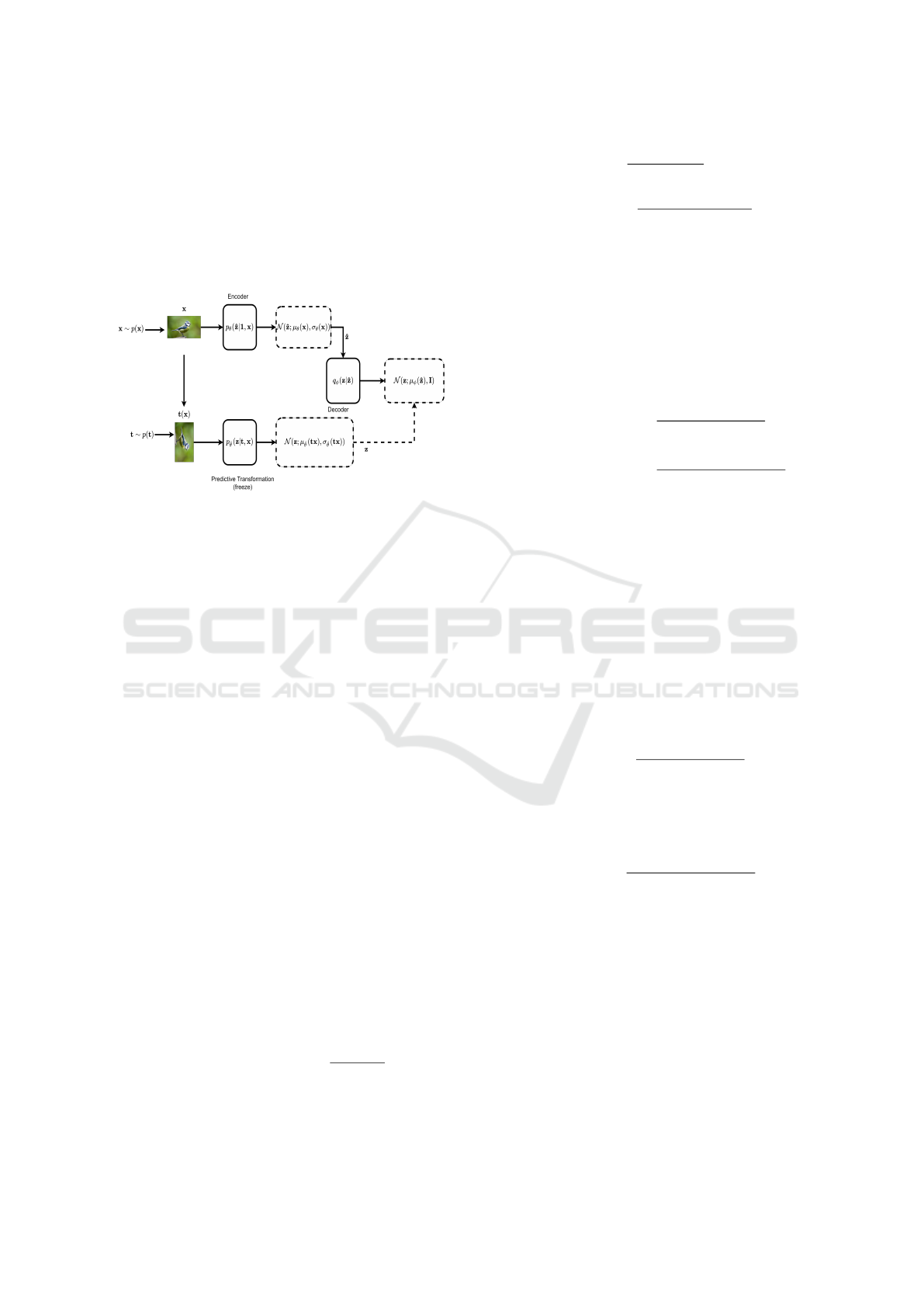
VTEBA as an autoencoder. Figure 3 shows the ar-
chitecture of VTEBA.
Figure 3: The architecture of VTEBA. The transformed im-
age is fed through the predictive-transformation’s encoder
p
ˆ
θ
, while the original images is fed through the encoder
p
θ
. The output of the encoder is the mean µ
θ
and the
standard-deviation σ
θ
. The representation
ˆ
z is sampled and
fed through the decoder q
φ
. The output of the decoder is the
mean µ
φ
, which corresponds to the representation of trans-
formed image z, obtained from p
ˆ
θ
.
The encoder E
θ
represents p
θ
(
ˆ
z|z). We assume that
p
θ
(
ˆ
z|z) is following a factored multivariate Gaussian
distribution N (
ˆ
z;µ
θ
, σ
θ
). Thus, the output of E
θ
is the
mean µ
θ
and the standard-deviation σ
θ
. The encoder
E
ˆ
θ
of the predictive-transformation is responsible to
infer z. Note that we freeze
ˆ
θ while training VTE. We
use the samples z to compute q
φ
(z|
ˆ
z). The decoder
D
φ
represents q
φ
(z|
ˆ
z) and takes
ˆ
z as the input. We
assume that q
φ
(z|
ˆ
z) is following N (z; µ
φ
, I) to reduce
the complexity of the model. Therefore, the output of
D
φ
is the mean µ
φ
.
3.4 InfoNCE Lower Bound Estimation
The second estimation method is the InfoNCE. Note
that we still utilize the predictive-transformation to in-
fer z. This method adopts the notion of contrastive
learning to estimate MI. Recall that from Equation 1,
we have the MI as the expectation of a density ratio
between conditional distribution and the marginal dis-
tribution. Given I
θ,
ˆ
θ
(
ˆ
z;z), then:
I
θ,
ˆ
θ
(
ˆ
z;z) = E
p
θ,
ˆ
θ
(t,
ˆ
z,z)
log
p
θ,
ˆ
θ
(
ˆ
z|z)
p(
ˆ
z)
(9)
Furthermore, suppose that we have a batch of sam-
ples {(
ˆ
z
i
, z
i
)}
N
i=1
. For a particular pair (
ˆ
z
i
, z
i
), we can
model the density ratio
p
θ,
ˆ
θ
(
ˆ
z=
ˆ
z
i
|z=z
i
)
p(
ˆ
z=
ˆ
z
i
)
as:
exp( f (
ˆ
z
i
, z
i
)) ∝
p
θ,
ˆ
θ
(
ˆ
z =
ˆ
z
i
|z = z
i
)
p(
ˆ
z =
ˆ
z
i
)
(10)
with f is an estimator function that takes (
ˆ
z
i
, z
i
) as the
input. Note that this approximation form can be un-
normalized, which means that the integral of the den-
sity ratio does not have to be 1. Therefore, for each
pair of (
ˆ
z
i
, z
i
), we normalize it by a partition func-
tion that takes the sum of (
ˆ
z
j
, z
i
), 1 ≤ j ≤ N ∧ i 6= j.
We call (
ˆ
z
i
, z
i
) a positive pair, while (
ˆ
z
j
, z
i
) a negative
pairs. Mathematically, we have
I
θ,
ˆ
θ
(
ˆ
z, z) ≥ E
∏
j
p
θ,
ˆ
θ
(t,
ˆ
z,z)
log
exp( f (
ˆ
z
i
, z
i
))
∑
ˆ
z
j
exp( f (
ˆ
z
j
, z
i
))
(11)
≥ E
∏
j
p
θ,
ˆ
θ
(t,
ˆ
z,z)
log
exp(g(
ˆ
z
i
)
T
h(z
i
))
∑
ˆ
z
j
exp(g(
ˆ
z
j
)
T
h(z
i
))
(12)
It is known that neural network is an universal approx-
imation for any function (Heaton, 2018). Therefore,
we implement the estimator function f as neural net-
work. We call this model as VTEInfoNCE concate-
nated version. Furthermore, we can decompose the
function f into two different functions g and h, each
takes
ˆ
z and z as input separately. We combine the
output by performing vector multiplication. We call
this model as VTEInfoNCE separated version. Let
ˆ
φ
be the parameter of estimator function f . The objec-
tive function of VTEInfoNCE concatenated version is
maximizing
max
θ,
ˆ
φ
E
∏
j
p
θ,
ˆ
θ
(t,
ˆ
z,z)
log
exp( f (
ˆ
z
i
, z
i
))
∑
ˆ
z
j
exp( f (
ˆ
z
j
, z
i
))
(13)
Subsequently, let
˜
φ, φ
0
be the parameter of the estima-
tor function g and h, respectively. The VTEInfoNCE
separated version aims to maximize
max
θ,
˜
φ,φ
0
E
∏
j
p
θ,
ˆ
θ
(t,
ˆ
z,z)
log
exp(g(
ˆ
z
i
)
T
h(z
i
))
∑
ˆ
z
j
exp(g(
ˆ
z
j
)
T
h(z
i
))
(14)
Note that we do not optimize the parameter
ˆ
θ. In the
next subsection, we provide the algorithm to train the
predictive-transformation and the VTE models. Fig-
ure 4 shows the architecture of VTEInfoNCE sepa-
rated.
3.5 Algorithm
3.5.1 Training Predictive-transformation
Suppose that we have a batch consists of N sam-
ples X =
x
i
N
i=1
. For each sample, we draw a
Transformation-Equivariant Representation Learning with Barber-Agakov and InfoNCE Mutual Information Estimation
103
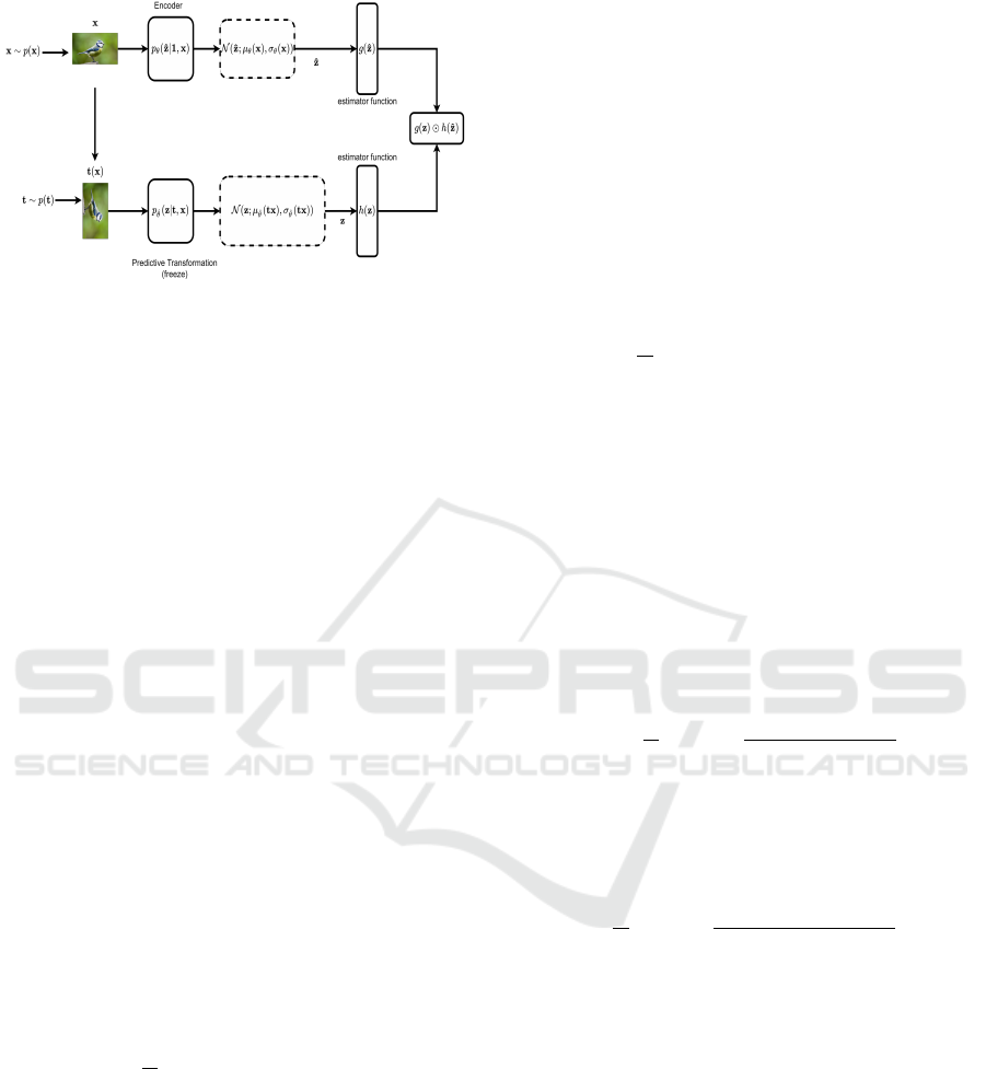
Figure 4: The architecture of VTEInfoNCE. The decoder is
replaced with estimator functions g and h, parameterized by
˜
φ and φ
0
, respectively.
transformation t
i
from p(t). We infer p
ˆ
θ
(z
i
|t
i
x
i
) by
feeding t
i
x
i
through encoder E
ˆ
θ
. Note that the out-
put of E
ˆ
θ
is the parameters of a probability distri-
bution. Therefore, we need to sample from the dis-
tribution to get z
i
instance. However, performing
ordinary sampling leads the model to fail to com-
pute the gradient of the objective function w.r.t. the
parameter
ˆ
θ (encoder parameter). This condition is
undesirable if we perform the optimization through
gradient-based method. Therefore, we apply the
reparameterization trick to solve the problem. This
trick is renowned used by the variational autoencoder
(Kingma and Welling, 2013). Given the mean µ
ˆ
θ
(t
i
x
i
)
and standard-deviation σ
ˆ
θ
(t
i
x
i
), we can write repa-
rameterization trick as:
z
i
= µ
ˆ
θ
(t
i
x
i
) + σ
ˆ
θ
(t
i
x
i
) ε
i
(15)
with denotes the pointwise multiplication. Recall
that µ and σ are obtained from the encoder E
ˆ
θ
. Fur-
thermore, ε
i
refers to a noise sampled from N (ε; 0, I).
Decoder D
ˇ
φ
takes z to output q
ˇ
φ
(t|z). Since we only
have the samples z, we translate the expectation into
an unbiased Monte Carlo estimation:
min
ˆ
θ,
ˇ
φ
1
N
N
∑
i=1
−log N (t
i
;µ
ˇ
φ
(z
i
), I) (16)
By the property of the monotonic function (log), we
minimize the negative of the objective function. Fur-
thermore, the decoder D
ˇ
φ
only outputs µ
ˇ
φ
(by the as-
sumption of q
ˇ
φ
(t|z)).
3.5.2 Training Variational
Transformation-Equivariant
We follow the same settings as the predictive-
transformation. Given samples X =
{
x
i
}
N
i=1
, we draw
transformation t
i
from p(t) for each x
i
. Subsequently,
we use encoder E
θ
to infer p
θ
(
ˆ
z
i
|x
i
). and perform the
reparameterization trick to generate
ˆ
z.
ˆ
z
i
= µ
θ
(x
i
) + σ
θ
(x
i
)
ˆ
ε
i
(17)
The noise
ˆ
ε is drawn from a standard Gaussian distri-
bution N (
ˆ
ε;0, I).
We use the encoder E
ˆ
θ
to infer p
ˆ
θ
(z
i
|t
i
). Note that
E
ˆ
θ
is the encoder of predictive-transformation. We
freeze the parameter
ˆ
θ since we do not optimize
ˆ
θ.
For the Barber-Agakov MI-estimation, we minimize
min
θ,φ
1
N
N
∑
i=1
−log N (z
i
;µ
φ
(
ˆ
z
i
), σ(
ˆ
z
i
)) (18)
Here we translate the expectation into an unbiased
Monte Carlo estimation method since we only have
the samples of
ˆ
z and z. We take the benefit of the
monotonic function’s property by translating the ob-
jective function into a minimization problem. De-
coder D
φ
represents q
φ
(z|
ˆ
z). By the assumption of
q
φ
(z|
ˆ
z), D
φ
only outputs the mean µ
φ
.
For the InfoNCE MI-estimation, we have two ver-
sions: the concated version and the separated version.
The objective function of the concatenated version is
as follows:
min
θ,
ˆ
φ
1
N
N
∑
i=1
−log
exp( f (
ˆ
z
i
, z
i
))
∑
ˆ
z
j
exp( f (
ˆ
z
j
, z
i
))
(19)
ˆ
φ denotes the parameter of estimator function f . Sub-
sequently, the objective function of the separated In-
foNCE is as follows:
min
θ,
˜
φ,φ
0
1
N
N
∑
i=1
−log
exp(g(
ˆ
z
i
)
T
h(z
i
))
∑
ˆ
z
j
exp(g(
ˆ
z
j
)
T
h(z
i
))
(20)
˜
φ, φ
0
denote the parameters of g and h, respec-
tively. Both VTEBA and VTEInfoNCE can utilize a
gradient-based method to optimize the objective func-
tion.
The difference between AVT and VTE lies in their
output. The decoder of AVT estimates the proba-
bility distribution p
θ
(t|
ˆ
z, z) through Barber-Agakov
MI estimation. On the other hand, the decoder of
VTEBA and the estimator function of VTEInfoNCE
aim to estimate p
θ
(
ˆ
z|z) through Barber-Agakov esti-
mation and noise contrastive loss, respectively. As a
result, AVT takes z and
ˆ
z as the inputs, while VTEBA
only takes one of either
ˆ
z or z. Furthermore, AVT re-
quires one stage of training while VTE requires two
stages of training. The latter is because VTE needs the
predictive-transformation model as the inductive bias,
ICPRAM 2022 - 11th International Conference on Pattern Recognition Applications and Methods
104
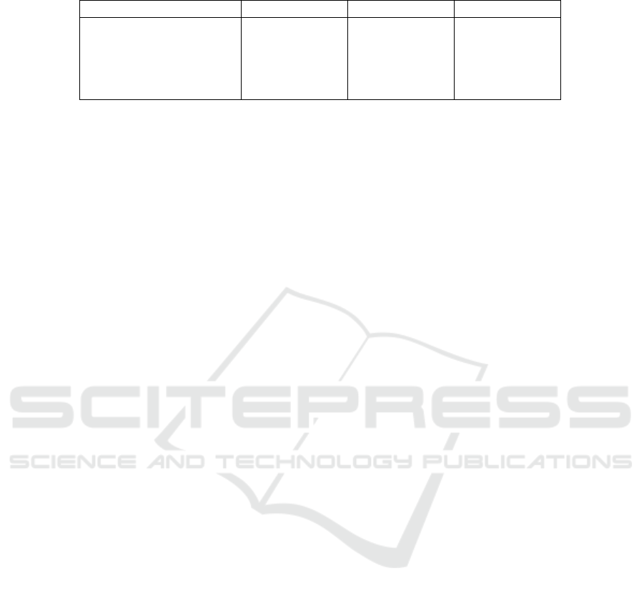
Table 1: The comparison of average error rate by different of each model with the various number of training data on CIFAR-
10 image classification using MLP.
Model 50K 5K 0.5K
AVT 0.147 ± 0.0001 0.355 ± 0.0018 0.797 ± 0.0021
predictive-transformation 0.142 ± 0.0006 0.383 ± 0.0028 0.655 ± 0.0036
VTEBA 0.140 ± 0.0000 0.354 ± 0.0001 0.508 ± 0.0006
VTEInfoNCE (1) 0.148 ± 0.0005 0.310 ± 0.0015 0.550 ± 0.0015
VTEInfoNCE (2) 0.152 ± 0.0000 0.362 ± 0.0016 0.476 ± 0.0006
which requires separate training. From the optimiza-
tion side, VTE and AVT depend on the gradient-based
method and reparameterization trick to optimize their
parameters.
4 EXPERIMENTS
For the experiments, we train predictive-
transformation, VTEBA, VTEInfoNCE separated
version, and VTEInfoNCE concatenated version. We
also reproduce AVT to give a fair comparison. We
then evaluate each of model on image classification
tasks. We utilize multi-layer perceptron (MLP),
K-nearest neighbor (K-NN), and multinomial logistic
regression as the classifiers. In this experiment, we
use CIFAR-10 (Krizhevsky et al., 2009) and STL-10
(Coates et al., 2011) datasets.
4.1 CIFAR-10 Experiment
Architecture. We follow the original architecture
of AVT for each model. Specifically, we use
Network-In-Network architecture (Lin et al., 2013)
for the convolution blocks (encoder). We represent
the distribution of z and
ˆ
z as a MLP of size 1024.
The first 512 neurons represent the mean and the
rest represent the log variance. The idea of replac-
ing the standard-deviation with the log variance is
to preserve numerical stability. We can derive the
standard-deviation by performing an exponentiation
trick. We implement the Decoder D
ˇ
φ
, D
φ
, and the es-
timator function f , g and h as MLP with three layers.
Implementation Details. All models are optimized
by adaptive moment (Adam) (Kingma and Ba, 2015)
with a learning rate of 1e − 4. We train the models
for 200 epochs. For each iteration, we chunk the data
into several mini-batches, each with size 256. We uti-
lize 1 GPU Tesla V-100 as the source of computation.
Furthermore, our models follow the same settings as
AVT (Qi et al., 2019) for the type of transformation.
For each image, we apply the projective transforma-
tion consists of random translation along horizontal
line and vertical line by [−0.125, 0.125] of the width
and the height of the image, random scaling with the
ratio [0.8, 1.2], and the random rotation with an angle
from {0
◦
, 90
◦
, 180
◦
, 270
◦
}.
Evaluation. We perform image classifications to
evaluate the models. First, we feed the feature ex-
tracted by the encoder of each model through an
MLP-based classifier. The MLP consists of three
fully connected layers. The first two layers share the
exact size of 2048 neurons, while the last layer has a
size of 10. We train the classifier on the various num-
ber of training data. Specifically, we train the MLP
on 50000, 5000, and 500 training data, respectively.
We then test the MLP on 10000 images. Since the
encoder is a probabilistic model, we perform the clas-
sification 5 times for each image and take the average
of the error rate. This approach is a bit different with
AVT since they only compute the error once.
Table 1 shows the classification results using MLP
on CIFAR-10 dataset. VTEInfoNCE (1) and VTE-
InfoNCE (2) refer to VTEInfoNCE separated ver-
sion and VTEInfoNCE concatenated version, respec-
tively. The results show that VTEBA outperforms the
other models on 50000 data with a 0.14 average er-
ror rate while VTEInfoNCE (2) gives the worst re-
sult. On 5000 data, VTEInfoNCE (1) outperforms
the others with a 0.31 ± 0.0015 average error rate,
while VTEInfoNCE (2) gives the worst result with a
0.355 ± 0.00018 average error rate. Finally, VTEIn-
foNCE (2) yields the best result with a 0.476±0.0006
average error rate on 500 data, while AVT yields the
worst result with a 0.797 ± 0.0021 average error rate.
In this experiment, the best model is different for each
number of data involved during the training. In gen-
eral, the proposed models give more satisfying results
compared to the baseline model.
Subsequently, we perform image classification
task by using K-NN. In this experiment, we choose
K = 5. All neighbors have an equal impact on the
classification result. Table 2 shows the classification
results using K-NN on CIFAR-10 dataset. From the
table, VTEBA consistently outperforms other mod-
els for every number of dataset. Furthermore, AVT
Transformation-Equivariant Representation Learning with Barber-Agakov and InfoNCE Mutual Information Estimation
105
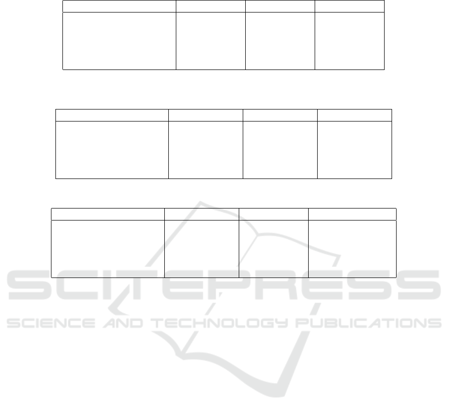
Table 2: The comparison of average error rate by different of each model with the various number of training data on CIFAR-
10 image classification using K-NN.
Model 50K 5K 0.5K
AVT 0.693 ± 0.050 0.743 ± 0.006 0.803 ±0.009
predictive-transformation 0.527 ± 0.006 0.596 ± 0.002 0.69 ± 0.011
VTEBA 0.396 ± 0.003 0.488 ± 0.003 0.578 ± 0.008
VTEInfoNCE (1) 0.429 ± 0.030 0.508 ± 0.004 0.583 ± 0.004
VTEInfoNCE (2) 0.448 ± 0.003 0.519 ± 0.001 0.596 ± 0.006
Table 3: The comparison of average error rate by different of each model with the various number of training data on CIFAR-
10 image classification using multinomial logistic regression.
Model 50K 5K 0.5K
AVT 0.622 ± 0.0023 0.759 ± 0.0023 0.840 ± 0.0029
predictive-transformation 0.539 ± 0.0025 0.698 ± 0.0018 0.793 ± 0.0046
VTEBA 0.391 ± 0.0005 0.457 ± 0.0003 0.603 ± 0.0003
VTEInfoNCE (1) 0.439 ± 0.0010 0.550 ± 0.0014 0.681 ± 0.0012
VTEInfoNCE (2) 0.423 ± 0.0015 0.523 ± 0.0011 0.656 ± 0.0028
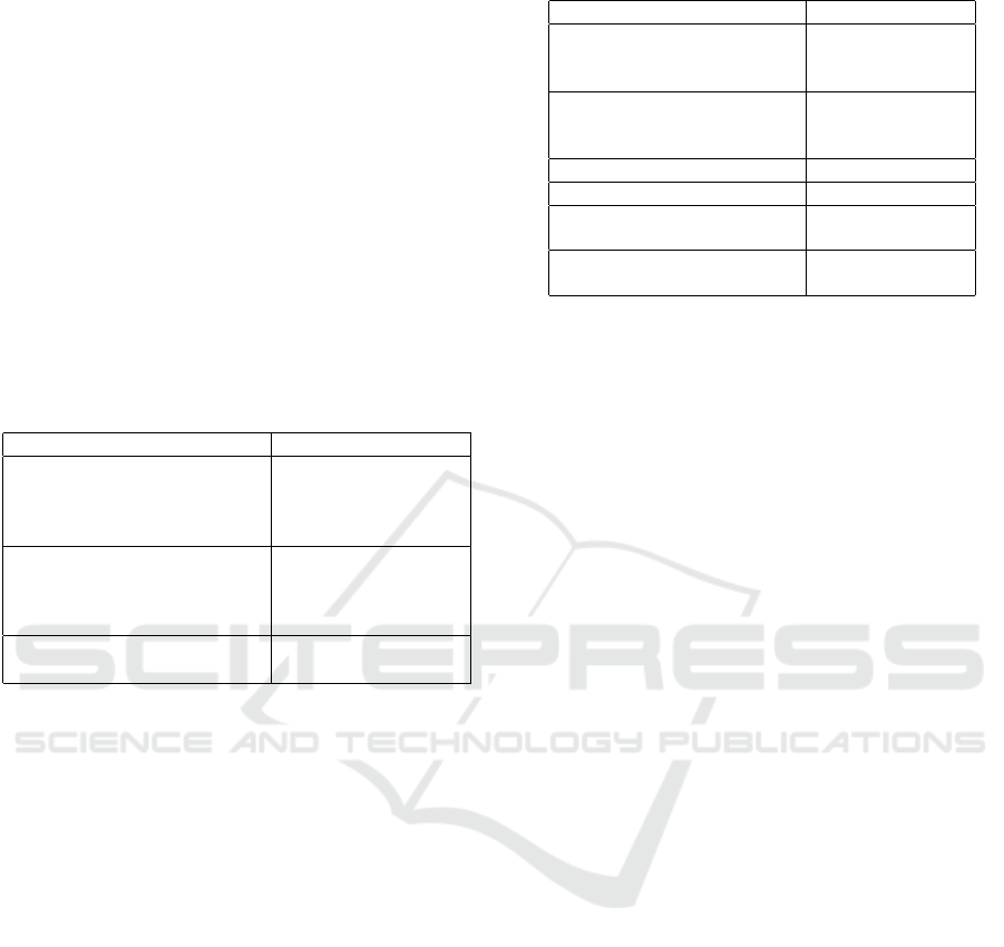
Table 4: Average error rate on STL-10 dataset using different classifiers.
Model PLB K-NN Logistic regression
AVT 0.522 ± 0.0000 0.707 ± 0.004 0.632 ± 0.0000
predictive-transformation 0.492 ± 0.0009 0.711 ± 0.002 0.544 ± 0.0012
VTEBA 0.460 ± 0.0007 0.607 ± 0.004 0.54 ± 0.0002
VTEInfoNCE (1) 0.365 ± 0.0000 0.475 ± 0.005 0.477 ± 0.0000
VTEInfoNCE (2) 0.363 ± 0.0005 0.473 ± 0.003 0.462 ± 0.0003
yields the highest average error rate for every number
of dataset.
Finally, we evaluate the representation models us-
ing multinomial logistic regression. The classifier op-
timize the cross-entropy loss for 100 iterations using
stochastic average gradient descent (SAG) (Schmidt
et al., 2017). Furthermore, we involve l
2
−norm to
regularize the weights of classifier. Table 3 shows
the classification results using multinomial logistic re-
gression on CIFAR-10 dataset. We have VTEBA con-
sistently outperforms other models for every number
of dataset. Moreover, AVT also becomes the model
with the highest average error rate for every number
of dataset.
We argue that two main factors cause the incon-
sistency results in Table 5. The first factor is the ten-
dency of MLP to suffer from over-fitting, especially if
there is only a small amount of data. The second fac-
tor is related to the characteristic of the representation
generated by VTEBA and VTEInfoNCE. We argue
that the contrastive loss leads VTEInfoNCE to gen-
erate representations that lie sparsely one each other.
On the other hand, the objective function of VTEBA
does not consider the relation of the representation
with its negative samples. Thus, the generated rep-
resentations are naturally more dense one each other.
VTEInfoNCE has an advantage on the image classi-
fication task, which involves a small amount of data
since the sparsity might reduce the overfitting to some
degree. However, this model performs poorly if we
have a large dataset since the MLP has to find a more
complex hypothesis (large and sparse). VTEBA per-
forms worse than VTEInfoNCE on a small dataset
since the MLP can fit the data too well. On the
contrary, VTEBA can give a better result on a large
dataset since the representations are more concen-
trated in some regions of the representation space.
4.2 STL-10 Experiment
Architecture. For STL-10 experiment, we adopt
the Alexnet architecture (Krizhevsky et al., 2017) for
the convolution blocks (encoder). Each block com-
prises a convolution and ReLU layer, followed by
a pooling layer. For the mean and the standard-
deviation, we adopt the same settings as the previous
experiment.
Implementation Details. In this experiment, we
train the proposed models and baseline model on
100000 unlabeled images, each with size 96× 96. We
first resize each image to 32 × 32. Subsequently, we
ICPRAM 2022 - 11th International Conference on Pattern Recognition Applications and Methods
106

apply the same transformation as the previous exper-
iment. All models are trained for 200 epochs with a
512 batch size. Same as previous research, the models
use 1 GPU Tesla V-100. We use the adaptive moment
to optimize the model with a learning rate 1e-4.
Figure 5: The first row shows sample images of the STL-10
dataset. The images in the second row are obtained by ap-
plying projective transformation on images in the first row.
Evaluation. We use the encoder of each model to
extract the feature for the image classification task.
We train an MLP, K-NN, and multinomial logistic re-
gression on 5000 labeled images. All classifiers fol-
low the same settings as the previous experiment. Fi-
nally, we ask each classifier to predict the class of
8000 unseen images. We also compute the average
error rate instead of just the error rate. Table 4 shows
the image classification results on the STL-10 dataset.
The results show that VTEInfoNCE(2) yields the low-
est average error-rate for each classifier. Further-
more, AVT achieve the highest average error-rate
for each classifier. The results are quite surprising
since we expect that AVT outperforms the predictive-
transformation. Recall that the goal of AVT is to max-
imize E
p
ˆ
θ
(t,
ˆ
z,z)
q
φ
(t|
ˆ
z, z). We argue that combining z
and
ˆ
z directly to reconstruct t restricts the expressive
power of z and
ˆ
z mutually. Thus, it reduces the gener-
alization of the model to extract the representation. In
contrast, VTE models z and
ˆ
z independently, allow-
ing the representations to fully exploit the structure of
data tx and x, without losing the equivariant property.
5 CONCLUSIONS
In this research, we investigate the alternatives of
autoencoding variational transformation (AVT). We
call the models variational transformation-equivariant
(VTE). We find that training VTE directly fails in the
model to learn the representation of the data. The rea-
son is due to the absence of the prior/inductive bias
that gives the context of training. Instead, we pro-
pose training the model into two phases. In the first
phase, we build a probabilistic self-supervised learn-
ing model to learn the representation of the trans-
formed image. Theoretically, this model maximizes
the mutual information (MI) between the transforma-
tion and the representation of the transformed image.
We call the model predictive-transformation. In the
second phase of training, we build a representation
model that learns the representation of the original
image. In theory, we maximize MI between the rep-
resentation of the original image and the represen-
tation of the transformed image. We leverage the
previous model to obtain the representation of the
transformed image. However, computing MI directly
is intractable. Therefore, we utilize Barber-Agakov
and InfoNCE MI estimation method to maximize MI.
Barber-Agakov estimation approximates the true pos-
terior distribution with a variational distribution that
is easy to compute. We call the model VTEBArber-
Agakov. InfoNCE estimation method uses the deep
learning network as an estimator function of the den-
sity ratio. In this research, we propose two versions of
VTE with InfoNCE estimation. We call them VTEIn-
foNCE concatenated version and VTEInfoNCE sepa-
rated version. Furthermore, we evaluate the proposed
models and baseline on image classification tasks.
Results on CIFAR-10 and STL-10 datasets show that
our proposed models outperform the baseline.
ACKNOWLEDGEMENTS
We gratefully acknowledge the support of the
Tokopedia-UI AI Center of Excellence, Faculty of
Computer Science, University of Indonesia, for al-
lowing us to use its NVIDIA DGX-1 for running our
experiments.
REFERENCES
Agakov, D. B. F. (2004). The im algorithm: a variational
approach to information maximization. Advances in
neural information processing systems, 16(320):201.
Alemi, A. A., Fischer, I., Dillon, J. V., and Murphy,
K. (2017). Deep variational information bottleneck.
In 5th International Conference on Learning Rep-
resentations, ICLR 2017, Toulon, France, April 24-
26, 2017, Conference Track Proceedings. OpenRe-
view.net.
Cheng, P., Hao, W., Dai, S., Liu, J., Gan, Z., and Carin, L.
(2020). CLUB: A contrastive log-ratio upper bound
of mutual information. In Proceedings of the 37th In-
ternational Conference on Machine Learning, ICML
2020, 13-18 July 2020, Virtual Event, volume 119
of Proceedings of Machine Learning Research, pages
1779–1788. PMLR.
Coates, A., Ng, A. Y., and Lee, H. (2011). An analysis of
single-layer networks in unsupervised feature learn-
ing. In Gordon, G. J., Dunson, D. B., and Dud
´
ık, M.,
Transformation-Equivariant Representation Learning with Barber-Agakov and InfoNCE Mutual Information Estimation
107

editors, Proceedings of the Fourteenth International
Conference on Artificial Intelligence and Statistics,
AISTATS 2011, Fort Lauderdale, USA, April 11-13,
2011, volume 15 of JMLR Proceedings, pages 215–
223. JMLR.org.
Cohen, T. and Welling, M. (2016). Group equivariant con-
volutional networks. In Balcan, M. and Weinberger,
K. Q., editors, Proceedings of the 33nd International
Conference on Machine Learning, ICML 2016, New
York City, NY, USA, June 19-24, 2016, volume 48 of
JMLR Workshop and Conference Proceedings, pages
2990–2999. JMLR.org.
Cohen, T. S. and Welling, M. (2017). Steerable cnns.
In 5th International Conference on Learning Rep-
resentations, ICLR 2017, Toulon, France, April 24-
26, 2017, Conference Track Proceedings. OpenRe-
view.net.
Doersch, C., Gupta, A., and Efros, A. A. (2015). Unsuper-
vised visual representation learning by context predic-
tion. In 2015 IEEE International Conference on Com-
puter Vision, ICCV 2015, Santiago, Chile, December
7-13, 2015, pages 1422–1430. IEEE Computer Soci-
ety.
Donsker, M. D. and Varadhan, S. S. (1975). Asymptotic
evaluation of certain markov process expectations for
large time, i. Communications on Pure and Applied
Mathematics, 28(1):1–47.
Dosovitskiy, A., Fischer, P., Springenberg, J. T., Riedmiller,
M. A., and Brox, T. (2016). Discriminative unsu-
pervised feature learning with exemplar convolutional
neural networks. IEEE Trans. Pattern Anal. Mach. In-
tell., 38(9):1734–1747.
Gidaris, S., Singh, P., and Komodakis, N. (2018). Unsuper-
vised representation learning by predicting image ro-
tations. In 6th International Conference on Learning
Representations, ICLR 2018, Vancouver, BC, Canada,
April 30 - May 3, 2018, Conference Track Proceed-
ings. OpenReview.net.
Heaton, J. (2018). Ian goodfellow, yoshua bengio, and
aaron courville: Deep learning - the MIT press, 2016,
800 pp, ISBN: 0262035618. Genet. Program. Evolv-
able Mach., 19(1-2):305–307.
Hinton, G. E., Krizhevsky, A., and Wang, S. D. (2011).
Transforming auto-encoders. In Honkela, T., Duch,
W., Girolami, M. A., and Kaski, S., editors, Artifi-
cial Neural Networks and Machine Learning - ICANN
2011 - 21st International Conference on Artificial
Neural Networks, Espoo, Finland, June 14-17, 2011,
Proceedings, Part I, volume 6791 of Lecture Notes in
Computer Science, pages 44–51. Springer.
Kingma, D. P. and Ba, J. (2015). Adam: A method for
stochastic optimization. In Bengio, Y. and LeCun,
Y., editors, 3rd International Conference on Learn-
ing Representations, ICLR 2015, San Diego, CA, USA,
May 7-9, 2015, Conference Track Proceedings.
Kingma, D. P. and Welling, M. (2013). Auto-encoding vari-
ational bayes. arXiv preprint arXiv:1312.6114.
Krizhevsky, A., Hinton, G., et al. (2009). Learning multiple
layers of features from tiny images.
Krizhevsky, A., Sutskever, I., and Hinton, G. E. (2017). Im-
agenet classification with deep convolutional neural
networks. Commun. ACM, 60(6):84–90.
Lenssen, J. E., Fey, M., and Libuschewski, P. (2018). Group
equivariant capsule networks. In Bengio, S., Wallach,
H. M., Larochelle, H., Grauman, K., Cesa-Bianchi,
N., and Garnett, R., editors, Advances in Neural
Information Processing Systems 31: Annual Con-
ference on Neural Information Processing Systems
2018, NeurIPS 2018, December 3-8, 2018, Montr
´
eal,
Canada, pages 8858–8867.
Lin, M., Chen, Q., and Yan, S. (2013). Network in network.
arXiv preprint arXiv:1312.4400.
Nguyen, X., Wainwright, M. J., and Jordan, M. I. (2010).
Estimating divergence functionals and the likelihood
ratio by convex risk minimization. IEEE Trans. Inf.
Theory, 56(11):5847–5861.
Noroozi, M. and Favaro, P. (2016). Unsupervised learning
of visual representations by solving jigsaw puzzles.
In Leibe, B., Matas, J., Sebe, N., and Welling, M.,
editors, Computer Vision - ECCV 2016 - 14th Euro-
pean Conference, Amsterdam, The Netherlands, Octo-
ber 11-14, 2016, Proceedings, Part VI, volume 9910
of Lecture Notes in Computer Science, pages 69–84.
Springer.
Noroozi, M., Pirsiavash, H., and Favaro, P. (2017). Repre-
sentation learning by learning to count. In IEEE Inter-
national Conference on Computer Vision, ICCV 2017,
Venice, Italy, October 22-29, 2017, pages 5899–5907.
IEEE Computer Society.
Poole, B., Ozair, S., van den Oord, A., Alemi, A., and
Tucker, G. (2019). On variational bounds of mu-
tual information. In Chaudhuri, K. and Salakhutdi-
nov, R., editors, Proceedings of the 36th International
Conference on Machine Learning, ICML 2019, 9-15
June 2019, Long Beach, California, USA, volume 97
of Proceedings of Machine Learning Research, pages
5171–5180. PMLR.
Qi, G. (2019). Learning generalized transformation equiv-
ariant representations via autoencoding transforma-
tions. CoRR, abs/1906.08628.
Qi, G., Zhang, L., Chen, C. W., and Tian, Q. (2019). AVT:
unsupervised learning of transformation equivariant
representations by autoencoding variational transfor-
mations. In 2019 IEEE/CVF International Confer-
ence on Computer Vision, ICCV 2019, Seoul, Korea
(South), October 27 - November 2, 2019, pages 8129–
8138. IEEE.
Schmidt, M., Roux, N. L., and Bach, F. R. (2017). Minimiz-
ing finite sums with the stochastic average gradient.
Math. Program., 162(1-2):83–112.
van den Oord, A., Li, Y., and Vinyals, O. (2018). Repre-
sentation learning with contrastive predictive coding.
CoRR, abs/1807.03748.
Wang, D. and Liu, Q. (2018). An optimization view on
dynamic routing between capsules. In 6th Interna-
tional Conference on Learning Representations, ICLR
2018, Vancouver, BC, Canada, April 30 - May 3, 2018,
Workshop Track Proceedings. OpenReview.net.
Zhang, L., Qi, G., Wang, L., and Luo, J. (2019). AET vs.
AED: unsupervised representation learning by auto-
encoding transformations rather than data. In IEEE
ICPRAM 2022 - 11th International Conference on Pattern Recognition Applications and Methods
108
Conference on Computer Vision and Pattern Recogni-
tion, CVPR 2019, Long Beach, CA, USA, June 16-20,
2019. Computer Vision Foundation / IEEE.
APPENDIX
5.1 Models Architecture on CIFAR-10
Dataset
Table 5 shows the architecture being used to build
predictive-transformation, AVT, VTEBA, VTEIn-
foNCE separated, and VTEInfoNCE concatenated on
CIFAR-10 dataset. The architecture of the encoder
follows the implementation of Network-In-Network.
Table 5: Architecture being used on CIFAR-10 experiment.
Encoder Decoder, f , g, dan h
Block(3, 192, 5) Linear(512, 2048)
Block(192, 160, 1) ReLU
Block(160, 96, 1) Linear(2048, 512)
Max-Pool(3, 2, 1)
Block(96, 192, 5)
Block(192, 192)
Block(192, 8)
Avg-Pool(3, 2, 1)
µ
φ
→ Linear(512, 512)
logσ
φ
→ Linear(512, 512)
Block(in, out, kernel) is a module con-
sists of Conv2D(in, out, kernel, stride=1,
padding=(kernel - 1) // 2) → Batch Norm
2D → ReLU. Parameter in denotes the size of input
channel, out denotes the size of output channel, and
kernel denotes the size of kernel which owns the
same height and width.
5.2 Models Architecture on STL-10
Dataset
Tabel 6 shows architecture being used to build
predictive-transformation, AVT, VTEBA, and VTE-
InfoNCE on STL-10 dataset. In this experiment,
the encoder adopts architecture of Alexnet. Alex
Block(in, out, kernel, stride, padding) is
a module consists of Conv2D(in, out, kernel,
stride, padding) → ReLU.
Table 6: Architecture being used on STL-10 experiment.
Encoder Decoder, f , g, dan h
Alex-Block(3, 64, 11, 1, 2) Linear(512, 2048)
Max-Pool(3, 2, 0) BatchNorm
ReLU
Alex-Block(64, 192, 5, 1, 2) Linear(2048, 1024)
Max-Pool(3, 2, 0) BatchNorm
ReLU
Alex-Block(192, 384, 3, 1, 1) Linear(1024, 512)
Alex-Block(96, 192, 5)
Alex-Block(192, 192)
Max-Pool(3, 2, 0)
µ
φ
→ Linear(1024, 512)
logσ
φ
→ Linear(1024, 512)
Transformation-Equivariant Representation Learning with Barber-Agakov and InfoNCE Mutual Information Estimation
109
