
Towards Deep Learning-based 6D Bin Pose Estimation in 3D Scans
Luk
´
a
ˇ
s Gajdo
ˇ
sech
1,2 a
, Viktor Kocur
2,4 b
, Martin Stuchl
´
ık
1 c
, Luk
´
a
ˇ
s Hudec
3 d
and Martin Madaras
1,2 e
1
Skeletex Research, Slovakia
2
Faculty of Mathematics, Physics and Informatics, Comenius University Bratislava, Slovakia
3
Faculty of Informatics and Information Technologies, Slovak Technical University Bratislava, Slovakia
4
Faculty of Information Technology, Brno University of Technology, Czech Republic
Keywords:
Computer Vision, Bin Pose Estimation, 6D Pose Estimation, Deep Learning, Point Clouds.
Abstract:
An automated robotic system needs to be as robust as possible and fail-safe in general while having relatively
high precision and repeatability. Although deep learning-based methods are becoming research standard on
how to approach 3D scan and image processing tasks, the industry standard for processing this data is still
analytically-based. Our paper claims that analytical methods are less robust and harder for testing, updating,
and maintaining. This paper focuses on a specific task of 6D pose estimation of a bin in 3D scans. Therefore,
we present a high-quality dataset composed of synthetic data and real scans captured by a structured-light
scanner with precise annotations. Additionally, we propose two different methods for 6D bin pose estimation,
an analytical method as the industrial standard and a baseline data-driven method. Both approaches are cross-
evaluated, and our experiments show that augmenting the training on real scans with synthetic data improves
our proposed data-driven neural model. This position paper is preliminary, as proposed methods are trained
and evaluated on a relatively small initial dataset which we plan to extend in the future.
1 INTRODUCTION
Capturing a scene with 3D scanners is a standard for
automatized systems analyzing a scene. To pick me-
chanical parts from a bin by a robotic arm equipped
with a gripper, the parts need to be localized. First,
the localization of bin is essential to restrain the robot
from collisions. Then, the kinematics of the robot is
optimized for path planning. The problem of bin lo-
calization can be defined as a 6 DoF pose estimation
of a template 3D model of the bin in the 3D scan.
Nowadays, analytical methods are still the indus-
trial standard for the processing of 3D scans. On the
contrary, the academic and research standards have
evolved to data-driven or hybrid approaches. Ana-
lytical computation of bin transformation in captured
point clouds might be vulnerable to missing critical
information in the captured scans, like corners and
a
https://orcid.org/0000-0002-8646-2147
b
https://orcid.org/0000-0001-8752-2685
c
https://orcid.org/0000-0001-8556-8364
d
https://orcid.org/0000-0002-1659-0362
e
https://orcid.org/0000-0003-3917-4510
edges, yielding lower robustness than expected. The
computation precision of a hard-defined analytical al-
gorithm might be higher but at the cost of lower ro-
bustness if a key content is missing. In applications
of automated intelligent systems, it may be interest-
ing to lower its precision to increase the robustness
in some scenarios. The other possible approach is
to split the pipeline into two steps - the first part of
the pipeline orients on the robustness and raw data-
driven localization. The second part focuses on the
precision-based analytical solution starting from the
predicted pose estimations, thus having the robustness
properties inherited from the data-driven approach.
In this paper, we present a novel dataset contain-
ing high-quality real and synthetic 3D scans of dif-
ferent bins in various poses containing a variety of
items captured by structured light scanners. We pub-
lish the dataset
1
for further research. We propose
an analytical method and a conceptually simple deep
convolutional neural network for 6D bin pose estima-
tion. We experimentally evaluate it and show that our
network is more robust than the analytical method.
1
http://skeletex.xyz/portfolio/datasets
Gajdošech, L., Kocur, V., Stuchlík, M., Hudec, L. and Madaras, M.
Towards Deep Learning-based 6D Bin Pose Estimation in 3D Scan.
DOI: 10.5220/0010878200003124
In Proceedings of the 17th International Joint Conference on Computer Vision, Imaging and Computer Graphics Theory and Applications (VISIGRAPP 2022) - Volume 4: VISAPP, pages
545-552
ISBN: 978-989-758-555-5; ISSN: 2184-4321
Copyright
c
2022 by SCITEPRESS – Science and Technology Publications, Lda. All rights reserved
545

Our method achieves better accuracy than existing
6D pose estimation methods. We also show the in-
clusion of synthetic data into the training process is
beneficial. We experimentally verify that cases of
successful pose approximations done by our network
can be further refined in post-processing with iterative
closest point (ICP), substantially increasing the por-
tion of data with close-to-zero final error. We present
this work as a position paper. We nevertheless feel
that the preliminary results presented in this paper
show promise, and we intend to continue this research
by collecting a larger dataset and performing a more
thorough evaluation.
2 RELATED WORK
Finding the 6D pose of an object is one of the clas-
sical computer vision problems tackled using vari-
ous methods over the years. Existing algorithms for
images and point clouds categorize into two main
groups, analytical algorithms (Stein and Medioni,
1992; Katsoulas, 2003b), and data-driven algo-
rithms. Data-driven algorithms can be further split
into feature-based methods (Vidal et al., 2018; Drost
et al., 2010) and Deep Neural Networks (DNN)-based
methods (Park et al., 2019; Bukschat and Vetter,
2020).
On the one hand, the feature-based methods are
optimized using only the 3D object model, as they
match pairs of points between the model and the cap-
tured scene. DNN-based methods, on the other hand,
are trained on large sets of actual 3D scenes to gener-
alize the solution. Moreover, a hybrid method can be
composed of a sequence of data-driven steps and the
final analytical step, with the ICP-like methods being
the widely-used analytical post-processing step (Besl
and McKay, 1992; Xiang et al., 2017). BOP chal-
lenge is trying to capture the state-of-the-art in this
area, comparing traditional and data-driven methods
on benchmark datasets (Hoda
ˇ
n et al., 2020).
Even though the problem of finding 3D translation
and 3D rotation of rigid objects is very general, it is
nevertheless dependant on the input data. Most of the
widely adopted datasets consist of RGBD images of
textured objects with complex geometries from a sin-
gle device with known internal camera parameters.
2.1 Analytical and Feature-based
Methods
A traditional approach of registering objects has been
detecting the local descriptors combined into shape-
based primitives and searching for their correspond-
ing pairs on 3D CAD models. The simplest case is
Hough transform applied to detect lines (Katsoulas,
2003b). The efforts to enhance the algorithm to re-
duce the number of possible detections resulted in
specifying that lines have to be orthogonal to repre-
sent the shape borders (Katsoulas, 2003a).
Similar to Hough transform, the RANSAC algo-
rithm extracts the geometric description of the object
by fitting the corresponding shape primitives into the
3D data. The non-deterministic algorithm is used in
a sequence of standard steps. (Guo et al., 2020) en-
hance the algorithm by using shape primitives to ap-
proximate the objects. (Vock et al., 2019) propose to
reduce 3D points into point pair features (PPF). How-
ever, RANSAC usually ends with many false pos-
itives (e.g., floor points); therefore, an ICP is usu-
ally required for fine-tuning. PPFs are widely used
in literature to estimate object points in point cloud
or RGBD data (Drost et al., 2010; Vidal et al., 2018;
Guo et al., 2021).
2.2 Deep Neural Network-based
Methods
Some methods estimate 6D poses from a single RGB
image either directly by modifying an existing 2D ob-
ject detection framework (Bukschat and Vetter, 2020)
or by using a neural network to obtain 2D-3D corre-
spondences further used in a PnP solver to obtain the
final pose (Park et al., 2019; Zakharov et al., 2019).
In contrast to RGB data, the scanners utilized in our
work output only texture from a grayscale camera -
not color, limiting the application of related papers
even further.
RGB with depth information is also commonly
used as input for deep learning base pose estimation.
Several methods (Mitash et al., 2018; Hosseini Ja-
fari et al., 2019) use deep learning models to output
hypotheses which are then processed in a hypothesis
validation pipeline to obtain the final poses. Other
indirect methods use deep learning networks to out-
put keypoints (He et al., 2020) or object fragments
(Hoda
ˇ
n et al., 2020) which are then used in a PnP
solver to obtain the final poses.
Other deep learning approaches apply neural net-
works directly to compute the 6D pose. DenseFu-
sion (Wang et al., 2020) uses RGB information to ob-
tain segmentation masks of objects. These are used
to combine depth and RGB data to generate per-
pixel embeddings, which are then used to estimate
object poses in a voting scheme. An improved ver-
sion of the algorithm called MaskedFusion (Pereira
and Alexandre, 2020) improves accuracy by masking
non-relevant data.
VISAPP 2022 - 17th International Conference on Computer Vision Theory and Applications
546

Figure 1: In this work we present a novel dataset contain-
ing 520 real and 370 synthetic 3D scans of bins. (Left)
Synthetic sample. (Right) Real scan annotated by hand.
The ground truth transformations of bin 3D model into the
scanner-space is demonstrated by purple mesh.
These approaches are trained for specific objects
and require their 3D models to be available during
training. We aim to be able to estimate 6D poses of
arbitrary bin-shaped objects. The mentioned meth-
ods are thus not easily transferable to our scenario.
Moreover, the methods are usually trained for cam-
eras with specific internal parameters, a constraint we
aim to avoid in our work.
2.3 Pose Parameterization
The pose of a rigid object can be described with a pair
of a rotation matrix R ∈ SO(3) and a translation vec-
tor
~
t ∈ R
3
. The translation vector can usually be rep-
resented directly as an output of a neural network and
used in a loss function since the space R
3
has a direct
continuous representation. On the other hand, there
are no continuous representations of SO(3), making
it difficult for neural networks to learn such represen-
tations (Zhou et al., 2019).
Rotational matrices only have 3 degrees of free-
dom while having 9 elements. Constraining the ele-
ments directly during the training process is imprac-
tical, so an orthogonalization procedure must be uti-
lized (Zhou et al., 2019). Rotation can also be rep-
resented using different equivalent parameterizations
such as quaternions (Xiang et al., 2017; Wang et al.,
2020; Pereira and Alexandre, 2020) or axis-angle vec-
tors (Bukschat and Vetter, 2020).
Symmetric objects pose a specific problem for ro-
tation representation. Depending on the type of sym-
metry, multiple different rotation parameterizations
can be valid for the same pose. This might introduce
problems as some loss functions can then have un-
desirable multiple global minima. Some approaches
mitigate these issues for some types of symmetries by
using losses based on distances of sampled points on
object models (Xiang et al., 2017; Wang et al., 2020;
Pereira and Alexandre, 2020) A different approach
(Pitteri et al., 2019) proposes mapping all represen-
tations onto a single canonical representation used
during training. Some methods avoid these issues
altogether by not directly outputting the object pose
but calculating it indirectly from keypoints (He et al.,
2020) or object fragments (Hoda
ˇ
n et al., 2020).
3 DATASET
We have collected a new dataset consisting of both
real captures (scans) from Photoneo PhoXi structured
light scanner devices (Photoneo, 2017) annotated by
hand and synthetic samples produced by our gener-
ator. See Figure 1 for an example of both real and
synthetic 3D scanner captures of scenes composed of
mechanical parts in a bin from our dataset.
In comparison with existing datasets, some no-
table differences include:
• most of the captured bins are texture-less, made
from uniform, single-colored materials,
• all bins are of cuboid shape with different propor-
tions. Compared to objects with complex geom-
etry, bins consist of flat faces with edges, which
are not guaranteed to be seen in the capture due
to occlusion. Surface models of these bins are not
provided, just their approximate bounding boxes,
• PhoXi scanner provides high-resolution 3D ge-
ometry data, but no RGB data, with a rough and
noisy gray-scale intensity image being the closest
equivalent,
• captures come from different devices with various
intrinsic camera parameters. We aim to work di-
rectly on 3D point clouds, which contain these pa-
rameters implicitly as opposed to RGBD images.
The original scans contain various parameters,
such as gray-scale intensities and normals. We rely
only on 2D single-view maps of 3D coordinates in
2064 × 1544 resolution in our proposed approaches.
We use 80% as the training data, and the remaining
20% (every fifth sample) plus a unique set of indepen-
dently captured 49 samples (including 10 synthetic
samples) as a test set. Due to its currently limited size,
we recommend cross-validation instead of an explicit
train-validation split. We plan to add more samples
into the dataset, as we will further enhance our meth-
ods in the future.
4 BIN POSE ESTIMATION IN 3D
POINT CLOUD
The bin pose estimation is a computation process of
estimating a transformation matrix that maps coordi-
nates of a bin-space into a scanner-space. As outlined
Towards Deep Learning-based 6D Bin Pose Estimation in 3D Scan
547
in the previous sections, the specific task of bin pose
estimation differs in many key aspects from the gen-
eral task of 6D pose estimation. Therefore, we have
decided to propose also two methods for this task.
The first method is an analytical heuristic we have
developed, and the second is a CNN-based pose es-
timation method. We deliberately designed the meth-
ods to be conceptually simple to provide solid base-
lines without bells and whistles. The following sub-
sections describe the proposed methods. Evaluation
and comparison of results for a set of experiments are
in Section 5.
4.1 Analytical Edge-based Fitting
An analytical algorithm for pose estimation is com-
posed of a set of steps performed sequentially in the
pipeline. This four-step method assumes that the top
edges of the bin are closer to the camera than back-
ground objects, and at least a part of every top edge
can be seen.
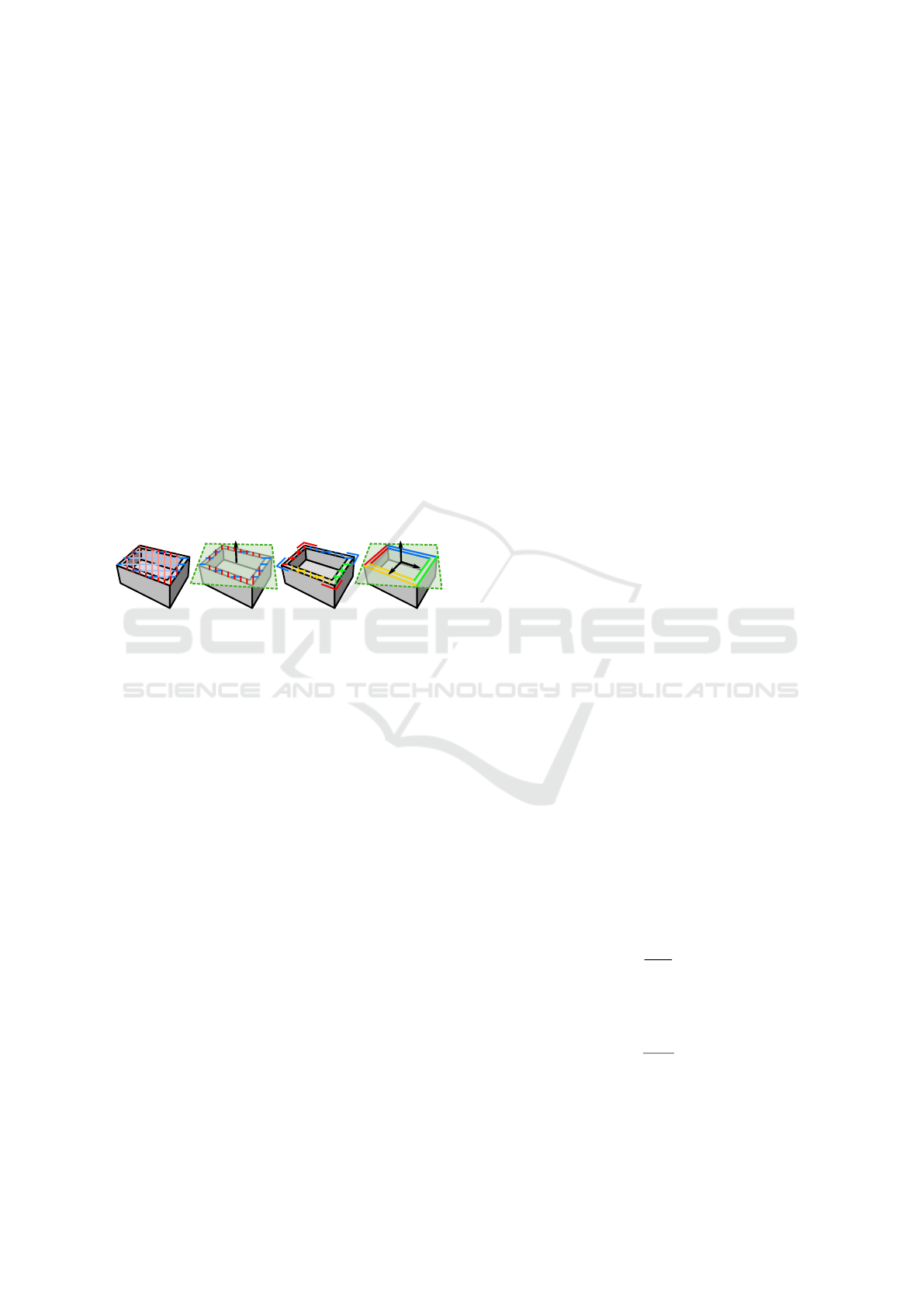
Figure 2: (From left to right) the camera space is row-wise
and column-wise segmented into similar depth intervals,
from which horizontal and vertical bin-cuts are constructed.
A plane is fitted into the bin-cuts, and wall-cuts not corre-
sponding to this plane are discarded as outliers. The re-
maining wall-cuts are assigned to four bin walls according
to corners fitted into horizontal and vertical bin-cuts. Fi-
nally, the lines are fitted into categorized wall-cuts, which
define the bin basis.
Initially, the horizontal and vertical scan-lines are
defined in scan-space. Each scan-line is divided into
intervals, where scan-line interval going through the
whole bin is called bin-cut. Specifically, each bin-cut
is composed of two wall-cuts and one interval for the
floor (representing the ground of the bin).
Next, minimum depth values in camera-space in
the intervals are detected, and vectors describing
edge-to-edge direction are computed. The set of such
vectors is computed in both directions, horizontally
and vertically (see Figure 2, left).
Moreover, a mode vector direction is computed in
both horizontal and vertical directions. Those mode
directions are used to compute the cross product of
these directions to compute the normal defining the
top of the bin. At the end of the step, the wall-cuts are
filtered according to the calculated plane.
Consequently, a corner detection is performed on
the filtered data. Each corner is detected as a bin-
cut endpoint, where the change of direction between
neighboring bin-cut endpoints is the highest; such de-
tection is performed in every direction, and all four
corners are detected (see Figure 2, right).
Finally, the set of detected corners categorizes
wall-cuts into four categories of the bin walls. Lines
are fitted into filtered wall-cuts, and the bin-space is
defined using the computed plane normal and fitted
lines, which can be used for the bin-space definition
and calculation of the final bin-space to camera-space
transformation.
4.2 CNN-based Pose Estimation
The analytical method may fail when bin edges or
corners are occluded or outside of the scanner view.
Such instances may frequently occur in industrial ap-
plications when human or robotic operators manipu-
late bins or contain items that cover the bin edges.
To overcome these issues, we propose a data-
driven approach using a convolutional neural net-
work. We propose a simple network that can reliably
estimate the pose up to a reasonable level of accuracy.
This estimate provided by the network is then refined
using an ICP algorithm to obtain the final bin pose.
4.2.1 Parameterization of the Bin Pose
The pose of the bin can be parameterized using a rota-
tion matrix R ∈ SO(3) and a translation vector
~
t ∈ R
3
.
We represent the translation vector directly. To repre-
sent rotation, we opt to use a strategy similar to (Zhou
et al., 2019) and represent the rotation by using two
vectors from R
3
which can be used to determine the
rotation matrix uniquely except for degenerate cases
discussed later. The two vectors represent the orien-
tation of the z and y axes of the bin in the camera
coordinates. We denote these vectors as ~v
z
and ~v
y
, re-
spectively.
To obtain the rotation matrix R from the vectors
~v
z
and ~v
y
, we employ the Gram–Schmidt orthogonal-
ization process to calculate the columns of the actual
rotation matrix they represent. During the procedure,
we perform the following calculations:
~u
z
=
~v
z
k~v
z
k
, (1)
~w
y
=~v
y
−
h
~v
y
|~u
z
i
~u
z
, (2)
~u
y
=
~w
z
k~w
z
k
, (3)
~u
x
=~u
y
×~u
z
. (4)
VISAPP 2022 - 17th International Conference on Computer Vision Theory and Applications
548
MLP
MLP
MLP
MLP
MLPMLP
ResNet
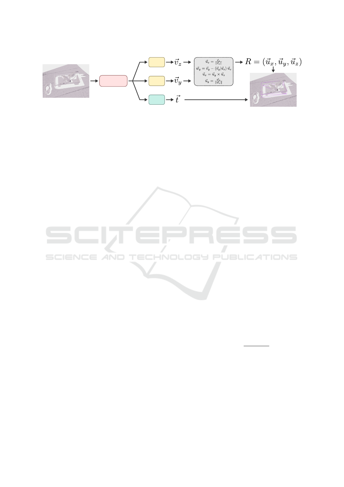
Figure 3: The architecture of the bin-pose estimation network. The structured point cloud is fed into a ResNet backbone. The
resulting features are fed into three separate heads. Each head is composed of a few fully-connected layers. One of the heads
outputs the resulting translation vector
~
t. The other two heads output intermediate vectors ~v
z
and ~u
z
. Equations (1-4) are then
used to obtain the columns of the resulting rotation matrix R.
The vectors ~u
x
,~u
y
,~u
z
form an orthonormal basis of
R
3
. We can then construct a matrix (~u
x
,~u
y
,~u
z
) which
is a valid rotation matrix. The fact that the matrix rep-
resents a proper rotation (e.g. det(R) = 1) is enforced
by equation (4).
Using this procedure, any two vectors ~u
z
and ~u
y
can yield a valid rotation matrix provided that they
are linearly independent. We found this limitation to
not be of concern in practice.
Under this parameterization, any rotation matrix
can be parameterized by many pairs of such vectors,
and it is thus not unique in this regard. However,
this is not an issue as we use a loss function which
only depends on orientations of ~u
z
and ~u
y
, which are
unique. To obtain a single pair of valid vectors ~u
z
and
~u
y
, which would yield a given matrix R, we can use
the third and second columns of the matrix.
4.2.2 Bin Symmetry
We aim to detect bins of rectangular shapes. Rect-
angular bins are symmetric in a 180-degree rotation
around an axis parallel to the bin-base normal going
through the center of the base. Therefore, there are
always two valid rotation matrices for each possible
bin pose, which introduces issues during training as
the network is forced to learn only one correct output
of two possible outputs for a similar input, resulting
in the network’s inability to converge.
To remedy this issue we employ a simple strategy.
The two possible rotations R
1
and R
2
are related by a
symmetry rotation (5) such that R
1
= R
s
R
2
, where
R
s
=
−1 0 0
0 −1 0
0 0 1
. (5)
Therefore, the only differences between the matrices
are the signs in the first two columns, which allows us
always to choose one of the matrices based on the sign
of the matrix elements. We always select the matrix
which has a positive element in the first row and sec-
ond column. If this element is zero, we use the sign of
the next element below. If the value is zero again, we
use the sign of the last row and second column, which
has to be 1 or -1.
4.2.3 Network Architecture
In our experiments we use a standard ResNet back-
bone (He et al., 2016) for feature extraction. We apply
global average pooling on the feature maps and feed
the resulting features into three separate branch-heads
to output the three vectors ~v
z
,~v
y
and
~
t. Each head
comprises two fully-connected layers, with ReLU ac-
tivations used in rotational heads and Leaky ReLU
activations used in the translational branch. The
whole network architecture, along with output post-
processing, is shown in Figure 3.
4.2.4 Loss Function
For a given ground truth pose defined by R and
ˆ
~
t we
first check whether to transform the rotation matrix
using R
s
as described in subsection 4.2.2. We extract
the vectors ~u
z
and ~u
y
as the third and second columns
of the rotation matrix. We then train the network,
which outputs three vectors ~u
z
,~u
y
,
~
t using a joint loss
function:
L = L
r
(~u
z
,~v
z
) + L
r
(~u
y
,~v
y
) + λL
L1
(
ˆ
~
t,
~
t), (6)
where L
L1
is the standard L1 loss, λ is a weight hy-
perparameter and L
r
is the angle between two vectors
in radians:
L
r
(~u,~v) = acos
h
~u|~v
i
k~ukk~vk + ε
, (7)
with ε added to prevent undefined loss for output vec-
tors with small norm.
5 EVALUATION AND FINAL
EXPERIMENTS
We evaluate the analytical method proposed in Sec-
tion 4.1 and the neural network described in Section
Towards Deep Learning-based 6D Bin Pose Estimation in 3D Scan
549

4.2 using the dataset described in Section 3. We also
show the results after refinement of the network out-
put with ICP and provide an experimental comparison
of our method to existing approaches.
5.1 Evaluation Metrics
Since we do not have 3D surface reconstruction of ev-
ery bin in our dataset, we rely on model-independent
pose error functions, i.e. comparing just the ground
truth
ˆ
P = (
ˆ
R,
ˆ
~
t ) and estimated P = (R,
~
t ) transforma-
tion matrices. All our ground-truth rotation matrices
consider the same orientation of the cuboid bin with
the longer dimension along the x-axis, therefore we
can use the strategy from subsection 4.2.2 to obtain
symmetries
ˆ
R
1
,
ˆ
R
2
and minimize the metrics. We plan
to complete the dataset with model reconstructions in
the future. This will allow the calculation of metrics
like e
ADI
,e
VSD
,e
MSSD
allowing for evaluation of the
actual surface alignment (Hinterstoißer et al., 2012).
Evaluating the translation
~
t is straight-forward us-
ing the euclidean distance e
TE
(
ˆ
~
t,
~
t ) = k
~
t −
ˆ
~
t k
2
. For
comparison of rotation, we use the angular distance
e
RE
(
ˆ
R,R), which is the angle between rotational axis
in angle-axis representation and can be directly com-
puted from the rotation matrices as:
e
RE
(
ˆ
R,R) = min
ˆ
R
0
∈{
ˆ
R
1
,
ˆ
R
2
}
arcos
Tr(
ˆ
R
0
R
−1
) − 1
2
!
, (8)
where Tr is the matrix trace operator.
5.2 Baseline Network Results
We have experimented with different configurations
of the proposed baseline network
2
, see Table 1 for re-
sults. Apart from the backbone, we tried two differ-
ent input resolutions, half and quarter of the raw scan,
which resulted in resolutions 1032 × 772 and 516 ×
386, respectively. ResNet18 with half-resolution of
the input scan has the worst performance, proba-
bly due to the small receptive field of the network.
Interestingly, ResNet34 with quarter-resolution out-
performed half-resolution. Additional sub-sampling
probably acted as a noise-suppression.
Additionally, we have trained the best performing
configuration on a subset of the dataset without the
synthetic samples. Naturally, it achieved the worst
test error since this set also contains synthetic scans,
which were not encountered during training. Surpris-
ingly, it also has higher errors e
TE
= 7.656, e
RE
=
0.559 on a subset of the test data with real samples
only. Configuration trained on both real and synthetic
2
https://github.com/gajdosech2/bin-detect
Table 1: Comparison of test errors of different configura-
tions. Column R denotes the fraction of raw scan resolution
used as network input. Column S denotes whether synthetic
samples were used during training.
Backbone R S L
z
r
L
y
r
e
TE
e
RE
ResNet18 1/4 3 0.058 0.198 3.808 0.256
ResNet34 1/4 3 0.057 0.145 3.469 0.197
ResNet18 1/2 3 0.070 0.249 5.791 0.234
ResNet34 1/2 3 0.063 0.222 3.979 0.266
ResNet34 1/4 7 0.042 0.281 5.379 0.323
samples achieves e
TE
= 6.108 and e
RE
= 0.529 on
such subset. This would suggest that the synthetic
data helps the model generalize on real scans, despite
the evident gap between real and synthetic samples.
Figure 4: (Left) final improvement of data-driven method
using ICP algorithm, (right) a fail-case of the ICP, where the
bin was snapped to ground points of the bin, worsening the
fit. Points of raw scan are in blue, prediction of the network
in pink and ICP refinement in green.
Apart from average values of metrics e
RE
,e
TE
, the
Table 1 also shows average losses L
z
r
= L
r
(~u
z
,~v
z
) and
L
y
r
= L
r
(~u
z
,~v
z
) over the validation set. The loss func-
tion has, in this case, useful interpretation even as an
evaluation metric. L
z
r
represents the error in the pre-
dicted normal of the bin’s bottom face, with L
y
r
denot-
ing the rotation around this axis.
A qualitative sample of the hybrid two-step ap-
proach, where the data-driven method is refined with
post-alignment using ICP, can be seen in Figure 4.
This refinement improved the results (both
e
TE
and
e
RE
) in 91 samples out of the 218 in validation + test
set. In general, it improves the pose estimation if the
bin model has exact size and walls are visible. How-
ever, as mentioned in Section 3, the dataset currently
does not contain complete surface reconstructions of
the bins, just their approximate bounding boxes.
Figure 5 shows the comparison between the base-
line network, its results after ICP refinement, the
same version trained over real data only, and our
analytical method. As can be seen, the analytical
method achieves reasonable error for approximately
40% samples. The remaining samples had either high
errors or the method failed to estimate in 47% cases,
which was treated as an infinite error. The ICP refine-
ment achieved almost zero error in a few cases. How-
VISAPP 2022 - 17th International Conference on Computer Vision Theory and Applications
550
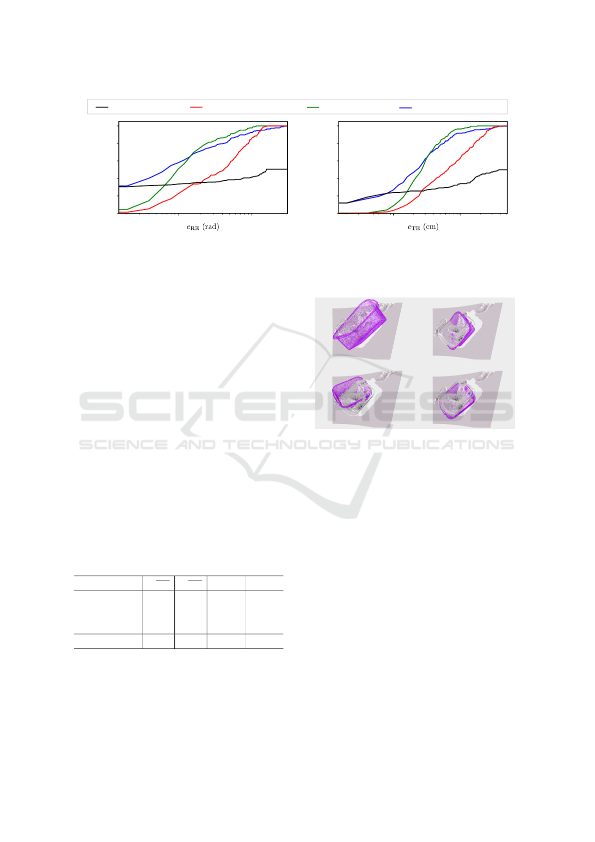
ResNet34 1/2 full + ICP
ResNet34 1/2 full
ResNet34 1/2 w/o synthAnalytical method
0.0
0.2
0.4
0.6
0.8
1.0
portion of samples
0.0
0.2
0.4
0.6
0.8
1.0
portion of samples
0.1 1.0 1.0 3.00.30.30.03 10.0 30.0
Figure 5: Vertical axes show the fraction of the test samples with the error below the value of the metrics e
RE
,e
TE
on the
horizontal axes. The analytical method achieves low error on a few samples but fails to predict pose for approximately half of
the cases. Using synthetic data in training improves the overall performance of the neural network. The hybrid method with
ICP refinement lowers the minimum error of the network, matching the analytical approach while also retaining robustness.
However, in some cases, the ICP fails to improve the bin pose, resulting in slightly increased overall maximum error.
ever, samples with non-corresponding points aligned
produced higher errors which can be improved by
limiting the usage of ICP only for confident cases,
where the number of paired-points is higher than
some threshold. This would mitigate the negative ef-
fect in a few cases, lowering the average error.
5.3 Comparison with Existing Methods
Despite the uniqueness of our data, we have trained
and qualitatively evaluated existing state of the art
models: DPOD (Zakharov et al., 2019), DenseFu-
sion (Wang et al., 2020), MaskedFusion (Pereira and
Alexandre, 2020) and EfficientPose (Bukschat and
Vetter, 2020). We performed the evaluation only on
a subset of our dataset (120 samples) with a single
bin model, for which we have made the required sur-
face reconstruction as the compared methods require
such data. See Figure 6 for qualitative comparison
and Table 2 for quantitative results over test set of 14
samples. We also show the performance of our pro-
posed baseline model.
Table 2: Results over small test set of 14 samples.
Model e
TE
e
RE
std e
TE
std e
RE
DenseFusion 7.544 0.493 2.473 0.364
MaskedFusion 6.583 0.494 2.145 0.361
EfficientPose 4.148 0.454 2.256 0.308
Ours 4.024 0.418 2.124 0.368
The scope of this experiment is limited, and
further evaluation is necessary to draw any strong
conclusions. However, this preliminary experiment
shows that our method can outperform the existing
ones while being conceptually simpler and not requir-
ing a model of the detected bin during training.
Figure 6: Qualitative comparison on single sample: Top
Left: DPOD, Top Right: EfficientPose, Bottom Left: Dense
Fusion, Bottom Right: Masked Fusion.
6 CONCLUSIONS AND FUTURE
WORK
In this paper, we have introduced a task of bin pose
estimation, which we identified as an essential com-
ponent in many vision-based automation systems in
the industry. We have collected a dataset of high-
quality 3D scans of various bins in different environ-
ments using scanners with various parameters. In our
future work, we aim to improve the dataset by collect-
ing more data to enable a more thorough evaluation of
bin pose estimation methods. We hope that such data
will be useful for further research in this area.
We also propose two baseline methods for 6D bin
pose estimation. The evaluation results suggest that
the bin poses can be estimated reliably with a sim-
ple convolutional neural network. In many cases, the
resulting poses can be further refined using ICP to im-
prove the accuracy of poses. We see the potential for
further research in this area, especially regarding the
Towards Deep Learning-based 6D Bin Pose Estimation in 3D Scan
551

effects of different types of bin pose parametrization
on the network performance.
ACKNOWLEDGEMENTS
The authors gratefully acknowledge the support of
NVIDIA Corporation with the donation of GPUs.
REFERENCES
Besl, P. and McKay, N. D. (1992). A method for registration
of 3-d shapes. IEEE Transactions on Pattern Analysis
and Machine Intelligence, 14(2):239–256.
Bukschat, Y. and Vetter, M. (2020). Efficientpose: An effi-
cient, accurate and scalable end-to-end 6d multi object
pose estimation approach.
Drost, B., Ulrich, M., Navab, N., and Ilic, S. (2010). Model
globally, match locally: Efficient and robust 3d object
recognition. In Proceedings of the IEEE Computer
Society Conference on Computer Vision and Pattern
Recognition, pages 998–1005.
Guo, J., Xing, X., Quan, W., Yan, D.-M., Gu, Q., Liu,
Y., and Zhang, X. (2021). Efficient center voting
for object detection and 6d pose estimation in 3d
point cloud. IEEE Transactions on Image Processing,
30:5072–5084.
Guo, N., Zhang, B., Zhou, J., Zhan, K., and Lai, S.
(2020). Pose estimation and adaptable grasp configu-
ration with point cloud registration and geometry un-
derstanding for fruit grasp planning. Computers and
Electronics in Agriculture, 179:105818.
He, K., Zhang, X., Ren, S., and Sun, J. (2016). Deep resid-
ual learning for image recognition. 2016 IEEE Con-
ference on Computer Vision and Pattern Recognition
(CVPR), pages 770–778.
He, Y., Sun, W., Huang, H., Liu, J., Fan, H., and Sun, J.
(2020). Pvn3d: A deep point-wise 3d keypoints voting
network for 6dof pose estimation.
Hinterstoißer, S., Lepetit, V., Ilic, S., Holzer, S., Brad-
ski, G. R., Konolige, K., and Navab, N. (2012).
Model based training, detection and pose estimation
of texture-less 3d objects in heavily cluttered scenes.
In ACCV.
Hoda
ˇ
n, T., Sundermeyer, M., Drost, B., Labb
´
e, Y., Brach-
mann, E., Michel, F., Rother, C., and Matas, J. (2020).
BOP challenge 2020 on 6D object localization. Euro-
pean Conference on Computer Vision Workshops (EC-
CVW).
Hoda
ˇ
n, T., Barath, D., and Matas, J. (2020). Epos: Estimat-
ing 6d pose of objects with symmetries. In Proceed-
ings of the IEEE/CVF Conference on Computer Vi-
sion and Pattern Recognition (CVPR), pages 11703–
11712.
Hosseini Jafari, O., Mustikovela, S. K., Pertsch, K., Brach-
mann, E., and Rother, C. (2019). ipose: Instance-
aware 6d pose estimation of partly occluded objects.
In Jawahar, C. V., Li, H., Mori, G., and Schindler, K.,
editors, Computer Vision – ACCV 2018, pages 477–
492, Cham. Springer International Publishing.
Katsoulas, D. (2003a). Localization of piled boxes by
means of the hough transform. In Joint Pattern Recog-
nition Symposium, pages 44–51. Springer.
Katsoulas, D. (2003b). Robust extraction of vertices in
range images by constraining the hough transform. In
IbPRIA, pages 360–369.
Mitash, C., Boularias, A., and Bekris, K. E. (2018). Im-
proving 6d pose estimation of objects in clutter via
physics-aware monte carlo tree search. In 2018 IEEE
International Conference on Robotics and Automation
(ICRA), pages 3331–3338.
Park, K., Patten, T., and Vincze, M. (2019). Pix2pose:
Pixel-wise coordinate regression of objects for 6d
pose estimation. 2019 IEEE/CVF International Con-
ference on Computer Vision (ICCV), pages 7667–
7676.
Pereira, N. and Alexandre, L. A. (2020). Maskedfusion:
Mask-based 6d object pose estimation.
Photoneo (2017). Phoxi 3d scanner. https://www.photoneo.
com/products/phoxi-scan-m/.
Pitteri, G., Ramamonjisoa, M., Ilic, S., and Lepetit, V.
(2019). On object symmetries and 6d pose estima-
tion from images. In 2019 International Conference
on 3D Vision (3DV), pages 614–622. IEEE.
Stein, F. and Medioni, G. (1992). Structural index-
ing: efficient 3-d object recognition. IEEE Transac-
tions on Pattern Analysis and Machine Intelligence,
14(2):125–145.
Vidal, J., Lin, C.-Y., Llado, X., and Mart
´
ı, R. (2018). A
method for 6d pose estimation of free-form rigid ob-
jects using point pair features on range data. Sensors,
18:2678.
Vock, R., Dieckmann, A., Ochmann, S., and Klein, R.
(2019). Fast template matching and pose estimation
in 3d point clouds. Computers & Graphics, 79:36–45.
Wang, C., Xu, D., Zhu, Y., Mart
´
ın-Mart
´
ın, R., Lu, C., Fei-
Fei, L., and Savarese, S. (2020). Densefusion: 6d ob-
ject pose estimation by iterative dense fusion.
Xiang, Y., Schmidt, T., Narayanan, V., and Fox, D. (2017).
Posecnn: A convolutional neural network for 6d ob-
ject pose estimation in cluttered scenes. arXiv preprint
arXiv:1711.00199.
Zakharov, S., Shugurov, I., and Ilic, S. (2019). Dpod: 6d
pose object detector and refiner. In International Con-
ference on Computer Vision (ICCV).
Zhou, Y., Barnes, C., Lu, J., Yang, J., and Li, H. (2019). On
the continuity of rotation representations in neural net-
works. In Proceedings of the IEEE/CVF Conference
on Computer Vision and Pattern Recognition, pages
5745–5753.
VISAPP 2022 - 17th International Conference on Computer Vision Theory and Applications
552
