
Improving the Sample-complexity of Deep Classification Networks with
Invariant Integration
Matthias Rath
1,2
and Alexandru Paul Condurache
1,2
1
Automated Driving Research, Robert Bosch GmbH, Stuttgart, Germany
2
Institute for Signal Processing, University of L
¨
ubeck, L
¨
ubeck, Germany
Keywords:
Geometric Prior Knowledge, Invariance, Group Transformations, Representation Learning.
Abstract:
Leveraging prior knowledge on intraclass variance due to transformations is a powerful method to improve the
sample complexity of deep neural networks. This makes them applicable to practically important use-cases
where training data is scarce. Rather than being learned, this knowledge can be embedded by enforcing in-
variance to those transformations. Invariance can be imposed using group-equivariant convolutions followed
by a pooling operation.
For rotation-invariance, previous work investigated replacing the spatial pooling operation with invariant inte-
gration which explicitly constructs invariant representations. Invariant integration uses monomials which are
selected using an iterative approach requiring expensive pre-training. We propose a novel monomial selection
algorithm based on pruning methods to allow an application to more complex problems. Additionally, we
replace monomials with different functions such as weighted sums, multi-layer perceptrons and self-attention,
thereby streamlining the training of invariant-integration-based architectures.
We demonstrate the improved sample complexity on the Rotated-MNIST, SVHN and CIFAR-10 datasets
where rotation-invariant-integration-based Wide-ResNet architectures using monomials and weighted sums
outperform the respective baselines in the limited sample regime. We achieve state-of-the-art results using full
data on Rotated-MNIST and SVHN where rotation is a main source of intraclass variation. On STL-10 we
outperform a standard and a rotation-equivariant convolutional neural network using pooling.
1 INTRODUCTION
Deep neural networks (DNNs) excel in problem set-
tings where large amounts of data are available such
as computer vision, speech recognition or machine
translation (LeCun et al., 2015). However, in many
if not most real-world problem settings training data
is scarce because it is expensive to collect, store and
in case of supervised training label. Consequently,
an important aspect of DNN research is to improve
the sample complexity of the training process, i.e.,
achieving best results when the available training data
is limited.
One solution to reduce the sample complexity is
to incorporate meaningful prior knowledge to bias the
learning mechanism and reduce the complexity of the
possible parameter search space. One well-known ex-
ample on how to embed prior knowledge are convo-
lutional neural networks (CNNs) which achieve state-
of-the-art performance in a variety of tasks related to
computer vision. CNNs successfully employ transla-
tional weight-tying such that a translation of the input
leads to a translation of the resulting feature space.
This property is called translation equivariance.
These concepts can be expanded such that they
cover other transformations of the input which lead to
a predictable change of the output – or to no change at
all. The former is called equivariance while the latter
is a related concept referred to as invariance.
In general, DNNs for image-based object detec-
tion and classification hierarchically learn a set of fea-
tures that ideally contain all relevant information to
distinguish different objects while dismissing the ir-
relevant information contained in the input. Gener-
ally, transformations causing intraclass variance can
act globally on the entire input image, e.g., global
rotations or illumination changes – or locally on the
objects, e.g., perspective changes, local rotations or
occlusions. Prior knowledge about those transforma-
tions can usually be obtained before training a DNN
and thus be incorporated to the training process or
architecture. Enforcing meaningful invariances on
214
Rath, M. and Condurache, A.
Improving the Sample-complexity of Deep Classification Networks with Invariant Integration.
DOI: 10.5220/0010872000003124
In Proceedings of the 17th International Joint Conference on Computer Vision, Imaging and Computer Graphics Theory and Applications (VISIGRAPP 2022) - Volume 5: VISAPP, pages
214-225
ISBN: 978-989-758-555-5; ISSN: 2184-4321
Copyright
c
2022 by SCITEPRESS – Science and Technology Publications, Lda. All rights reserved

the learned features simplifies distinguishing relevant
from irrelevant input information. One method to en-
force invariance is to approximately learn it via data
augmentation, i.e., artificially transforming the input
during training. However, these learned invariances
are not exact and do not cover all relevant variability.
(Cohen and Welling, 2016) first applied group-
equivariant convolutions (G-Convs) to DNNs. G-
Convs mathematically guarantee equivariance to
transformations which can be modeled as a group. A
DNN consisting of multiple layers is equivariant with
respect to a transformation group, if each of its lay-
ers is group-equivariant or commutes with the group
(Cohen and Welling, 2016). Consequently, an equiv-
ariant DNN consists of multiple group-convolutional
layers as well as pooling and normalization operations
that commute with the desired transformations. For
a classifier, the G-Convs are usually followed by a
global pooling operation over both the group dimen-
sion and the spatial domain in order to enforce invari-
ance. These invariant features are then processed by
fully connected layers to obtain the final class scores.
Invariant Integration (II) is a method to explicitly
create a complete, invariant feature space with respect
to a transformation group introduced by (Schulz-
Mirbach, 1992; Schulz-Mirbach, 1994). Recent work
showed that explicitly enforcing rotation-invariance
by means of II instead of using a global pooling
operation among the spatial dimensions decreases
the sample complexity of rotation-equivariant CNNs
used for classification tasks despite adding parame-
ters, hence improving generalization (Rath and Con-
durache, 2020). However, II thus far relies on cal-
culating monomials which are hard to optimize with
usual DNN training methods. Additionally, mono-
mial parameters have to be chosen using an iterative
method based on the least square error of a linear clas-
sifier before the DNN can be trained. This method re-
lies on an expensive pre-training step that reduces the
applicability of II to real-world problems.
Consequently, in this paper we investigate how
to adapt the rotation-II framework in combination
with equivariant backbone layers in order to reduce
the sample complexity of DNNs on various real-
world datasets while simplifying the training process.
Thereby, we explicitly investigate the transition be-
tween in- and equivariant features for the case of ro-
tations and replace the spatial pooling operation by II.
We start by introducing a novel monomial selection
algorithm based on pruning methods. Additionally,
we investigate replacing monomials altogether, using
simple, well-known DNN layers such as a weighted
sum (WS), a multi-layer perceptron (MLP) or self-
attention (SA) instead. This contributes significantly
to streamlining the entire framework. We specifically
apply these approaches to 2D rotation-invariance. We
achieve state-of-the-art results irrespective of limited-
or full-data regime, when rotations are responsible for
most of the relevant variability, such as on Rotated-
MNIST and SVHN. Furthermore, we demonstrate
very good performance in limited-data regimes on
CIFAR-10 and STL-10, when besides rotations also
other modes of intraclass variation are present.
Our core contributions are:
• We introduce a novel algorithm for the II mono-
mial selection based on pruning.
• We investigate various functions to replace the
monomials within the II framework including a
weighted sum, a MLP and self-attention. We
thereby streamline the training process of II-
enhanced DNNs as the monomial selection is no
longer needed.
• We demonstrate the performance of rotation-II
on the real world datasets SVHN, CIFAR-10 and
STL-10.
• We apply II to Wide-ResNet (WRN) architec-
tures, demonstrating its general applicability.
• We establish a connection between II and regular
G-Convs.
• We show that using II in combination with equiv-
ariant G-Convs reduces the sample complexity of
DNNs.
2 RELATED WORK
DNNs can learn invariant representations using
group-equivariant convolutions or equivariant at-
tention in combination with pooling operations.
Other methods explicitly learn invariance, or enforce
it using invariant integration.
Group-equivariant convolutional neural net-
works (G-CNNs) are a general framework to intro-
duce equivariance, first proposed and applied to 90
◦
rotations and flips on 2D images by (Cohen and
Welling, 2016). G-CNNs were extended to more fine-
grained or continuous 2D rotations (Worrall et al.,
2017; Bekkers et al., 2018; Veeling et al., 2018;
Weiler et al., 2018b; Winkels and Cohen, 2019; Di-
aconu and Worrall, 2019b; Walters et al., 2020), pro-
cessed as vector fields (Marcos et al., 2017) or fur-
ther generalized to the E(2)-group which includes
rotations, translations and flips (Weiler and Cesa,
2019). Additionally, 2D scale-equivariant group con-
volutions have been introduced (Xu et al., 2014;
Kanazawa et al., 2014; Marcos et al., 2018; Ghosh
and Gupta, 2019; Zhu et al., 2019; Worrall and
Improving the Sample-complexity of Deep Classification Networks with Invariant Integration
215

Group-Equivariant
Convolutions
Group
Max Pool
Invariant
Integration
Fully
Connected
Class Scores
Figure 1: General invariant DNN architecture using II. The architecture includes group convolutions (orange) and group
pooling (red) creating an equivariant representation, an II layer enforcing invariance (blue), and fully-connected layers (green).
Welling, 2019; Sosnovik et al., 2020). Further ad-
vances include expansions towards three-dimensional
spaces (e.g., (Worrall and Brostow, 2018; Kondor
et al., 2018; Esteves et al., 2018a)) or general man-
ifolds and groups (e.g., (Cohen et al., 2019a; Co-
hen et al., 2019b; Bekkers, 2020; Finzi et al., 2021))
which are beyond the scope of this paper.
Recently, equivariance was also introduced to at-
tention layers. (Diaconu and Worrall, 2019a; Romero
and Hoogendoorn, 2020; Romero et al., 2020) com-
bined equivariant attention with convolution layers to
enhance their expressiveness. (Fuchs et al., 2020;
Fuchs et al., 2021; Romero and Cordonnier, 2020;
Hutchinson et al., 2020) introduced different equiv-
ariant transformer architectures. In order to obtain in-
variant representations, equivariant layers are usually
combined with pooling operations.
Other methods to learn invariant representa-
tions include data augmentation, pooling over all
transformed inputs (Laptev et al., 2016), learning to
transform the input or feature spaces to their canon-
ical representation (Jaderberg et al., 2015; Esteves
et al., 2018b; Tai et al., 2019) or regularization meth-
ods (Yang et al., 2019). However, these methods ap-
proximate invariance rather than enforcing it mathe-
matically guaranteed.
Invariant integration is a principled method to
enforce invariance. It was introduced as a gen-
eral algorithm in (Schulz-Mirbach, 1992; Schulz-
Mirbach, 1994) and applied in combination with
classical machine learning classifiers for various
tasks such as rotation-invariant image classification
(Schulz-Mirbach, 1995), speech recognition (M
¨
uller
and Mertins, 2009; M
¨
uller and Mertins, 2010; M
¨
uller
and Mertins, 2011), 3D-volume and -surface classifi-
cation (Reisert and Burkhardt, 2006) or event detec-
tion invariant to anthropometric changes (Condurache
and Mertins, 2012).
In (Rath and Condurache, 2020), rotation-II was
applied in combination with steerable G-Convs in
DNNs for image classification. The equivariant fea-
ture space learned by the G-Convs is followed by
max-pooling among the group elements. Rotations
of the input induce rotations in the resulting feature
space, i.e., it is equivariant to rotations. While stan-
dard G-CNNs employ spatial max-pooling afterwards
to achieve an invariant representation, (Rath and Con-
durache, 2020) and our approach replace it with II,
which increases the expressibility compared to spatial
max-pooling while still guaranteeing invariant fea-
tures. These are finally processed with dense layers
to calculate the classification scores (see Figure 1).
All previous methods including (Rath and Con-
durache, 2020) used II in combination with mono-
mials which were either hand-designed or selected
using expensive iterative approaches which required
pre-training the entire network without II. In contrast,
we propose a novel pre-selection algorithm based on
pruning methods or to replace the monomials alto-
gether. Both approaches can be applied to DNNs
more natively.
3 PRELIMINARIES
In this section we concisely present the mathemati-
cal principles needed to define in- and equivariance
in DNNs which rely on Group Theory. Furthermore,
we introduce group-equivariant convolutions which
are used to obtain equivariant features and form the
backbone of our DNNs.
3.1 In- & Equivariance
A group G is a mathematical abstraction consisting
of a set X and a group operation · : G × G → G that
combines two elements to form a third. A group ful-
fills the four axioms closure, associativity, invertibil-
ity and identity. Group Theory is important for DNN
research, because invertible transformations acting on
feature spaces can be modeled as a group, where
the left group action G × R
n
→ R
n
,(g,x) 7→ L
g
x with
g ∈ G acts on the vector space R
n
.
The concept of in- and equivariance can be mathe-
matically defined on groups. A function f : R
n
→ R
m
is defined as equivariant, if its output f (x) transforms
VISAPP 2022 - 17th International Conference on Computer Vision Theory and Applications
216

predictably under group transformations
∀ g ∃ g
0
s.t. f (L
g
x) = L
g
0
f (x), (1)
for all x ∈ R
n
, and g ∈ G, g
0
∈ G
0
while G and G
0
may
be the same or different groups. If the output does
not change under transformations of the input, i.e.,
∀ g ∀ x, f (L
g
x) = f (x), f is invariant (Cohen and
Welling, 2016).
3.2 Group-equivariant Convolutions
(Cohen and Welling, 2016) first used the generaliza-
tion of the convolution towards general transforma-
tion groups G in the context of CNNs. The discrete
group-equivariant convolution of a signal x and a fil-
ter ψ : G → R
n
is defined as
[x ?
G
ψ](g) =
∑
h∈G
x(h)ψ(g
−1
h). (2)
Here, x : G → R
n
is used as a function. Both defini-
tions are interchangeable. The standard convolution
is a special case where G = Z
2
. The output of the
group-convolution is no longer defined on the regu-
lar grid, but on group elements g and is equivariant
w.r.t G. The action L
g
0
in the output space depends
on the group representation that is used. Two com-
mon representations used for G-CNNs are the irre-
ducible representation and the regular representation
which consists of one additional group channel per
group element storing the responses to all transformed
versions of the filters. Often, the regular representa-
tion is combined with transformation-steerable filters
which can be transformed arbitrarily via a linear com-
bination of basis filters, hence avoiding interpolation
artifacts (Freeman and Adelson, 1991; Weiler et al.,
2018b; Weiler et al., 2018a; Weiler and Cesa, 2019;
Ghosh and Gupta, 2019; Sosnovik et al., 2020). In
order to obtain invariant features from the equivari-
ant ones learned by G-CNNs, a pooling operation is
usually employed.
4 INVARIANT INTEGRATION
Invariant Integration introduced by (Schulz-Mirbach,
1992) is a method to create a complete feature space
w.r.t. a group transformation based on the Group Av-
erage A[ f ](x)
A[ f ](x) =
Z
g∈G
f (L
g
x)dµ(g), (3)
where
R
dµ(g) = 1 defines the Haar Measure and f
is an arbitrary complex-valued function. A complete
feature space implies that all patterns that are equiv-
alent w.r.t G are mapped to the same point while all
non-equivalent patterns are mapped to distinct points.
4.1 Monomials
For the choice of f , (Schulz-Mirbach, 1992) proposes
to use the set of all possible monomials which form a
finite basis of the signal space according to (Noether,
1916). Monomials are a multiplicative combination
of different scalar input values x
i
with exponents b
i
∈
R
m(x) =
M
∏
i=1
x
b
i
i
with
M
∑
i=1
b
i
≤ |G|. (4)
Combined with the finite group average, we obtain
A[m](x) =
1
|G|
∑
g∈G
m(L
g
x) =
1
|G|
∑
g∈G
M
∏
i=1
(L
g
x)
b
i
i
, (5)
(Schulz-Mirbach, 1994). When applying II with
monomials to two-dimensional input data on a regular
grid such as images, it is straightforward to use pixels
and their neighbors for the monomial factors x
i
. Con-
sequently, monomials can be defined via the distance
of the neighbor to the center pixel d
i
with d
1
= 0. For
discrete 2D rotations and translations, this results in
the following formula (Schulz-Mirbach, 1995)
A[m](x) =
1
UV Φ
∑
u,v,φ
M
∏
i=1
x[u+cos(φ)d
i
,v+sin(φ)d
i
]
b
i
, (6)
which can be used within a DNN with learnable ex-
ponents b
i
(Rath and Condurache, 2020).
4.2 Monomial Selection
While the II layer reduces the sample complexity
when learning invariant representations, it introduces
additional parameters which need to be carefully de-
signed. One of them is the selection of a meaningful
set of parameters d
i
and b
i
that define the monomi-
als needed to obtain the invariant representation. This
step is necessary since the number of possible mono-
mials satisfying
∑
i
b
i
≤ |G| is too extensive.
In (Rath and Condurache, 2020), an iterative ap-
proach is used based on the least square error solu-
tion of a linear classifier. While the linear classifier
is easy to compute, the iterative selection is time-
consuming and computationally expensive. Addition-
ally, the base network without the II layer needs to
be pre-trained which requires additional computations
and prevents training the full network from scratch.
Consequently, we investigate alternative ap-
proaches for the monomial selection. Two selection
approaches are introduced and explained in the fol-
lowing. Both enable training the network end-to-
end from scratch and are computationally inexpensive
compared to the iterative approach.
Improving the Sample-complexity of Deep Classification Networks with Invariant Integration
217

4.2.1 Random Selection
First, we randomly select the n
m
monomials by sam-
pling both the exponents and the distances from uni-
form distributions. This approach is fast only requir-
ing a single random sampling operation and serves as
a baseline to evaluate other selection methods.
4.2.2 Pruning Selection
Alternatively, monomial selection can be formulated
as selecting a subset containing n
m
M possible
monomial parameters. Consequently, it is closely re-
lated to the field of pruning in DNNs whose goal is to
reduce the amount of connections or neurons within
DNN architectures in order to reduce the computa-
tional complexity while maintaining the best possible
performance. We compare two pruning algorithms: a
magnitude- and a connectivity-based approach.
Magnitude-based Approach. (Han et al., 2015) de-
termine the importance of connections in DNNs by
pre-training the network for τ epochs and sorting
the weights of all layers by their magnitude |w
i j
|.
This approach is applied iteratively keeping the γ
highest-ranked connections at each step until the fi-
nal pruning-ratio γ
I
is reached.
Since we aim to prune monomials instead of sin-
gle connections, we sum the absolute value of weights
connected to a single monomial, i.e., all weights of
the first fully connected layer following the II layer:
s
j
=
1
C
i
C
o
C
i
∑
k=1
C
o
∑
l=1
|w
kl j
|, (7)
where C
i
is the number of input channels before II is
applied, C
o
is the number of neurons in the fully con-
nected layer and j selects the connections belonging
to the j
th
monomial. Following (Han et al., 2015), we
apply the pruning iteratively. In each step, we keep
the n
i
monomials with the highest calculated score
s
j
. We do not re-initialize our network randomly
in between iterative steps but re-load the pre-trained
weights from the previous step.
Connectivity-based Approach. We examine a sec-
ond pruning approach based on the initial connec-
tivity of weights inspired by (Lee et al., 2019). All
monomial output connections are multiplied with an
indicator mask c ∈ {0, 1}
M
using the Hadamard prod-
uct c w
l
. Here, w
l
is the weight vector of the fully
connected layer following the II step. Setting an indi-
vidual value c
j
to zero results in deleting all connec-
tions w
l, j
connected to monomial j. Consequently,
the effect of deactivating a monomial can be estimated
w.r.t the training loss L by calculating the connection
sensitivity
s
j
=
∂L(c, w
l
;D)
∂c
j
(8)
for each monomial using backpropagation. The n
m
monomials with the highest connection sensitivity are
kept. The derivative is calculated using the training
dataset D.
The connectivity-based approach can either be
used directly after initializing the DNN, or after some
pre-training steps. Additionally, it can either be used
iteratively or in a single step.
4.2.3 Initial Selection
We investigate two different approaches for the ini-
tial selection of M n
m
monomials. In addition to
a purely random selection, we design a catalog-based
initial selection in which all possible distance com-
binations are guaranteed to be involved in the initial
set. In both cases, we sample the exponents randomly
from a uniform distribution.
4.3 Replacing the Monomials
In addition to the novel monomial selection algo-
rithm, we investigate alternatives for the monomials
used to calculate the group average (Equation 3). We
apply the proposed functions to the group of discrete
2D rotations and compare monomials to well-utilized
DNN functions such as a weighted sum, a MLP and a
self-attention-based approach.
4.3.1 Weighted Sum
One possibility for f is to use a weighted sum where
the weights are a learnable kernel ψ applied at each
group element g transforming the input x. We obtain
A[WS](x) =
1
|G|
∑
g∈G
∑
y∈Z
2
x(y)ψ(g
−1
y). (9)
For 2D-rotations, this results in translating and rotat-
ing the kernel using all group elements g ∈ SO(2). We
implement two different versions of II with WS. First,
we apply a global convolutional filter, i.e., the kernel
size is equivalent to the size of the input feature map
(Global-WS). Secondly, we use local filters with ker-
nel size k which we apply at all spatial locations (u, v)
and all orientations φ (Local-WS).
Relation to Group Convolutions. In the following
we show the close connection between II using a WS
and the group convolution introduced by (Cohen and
Welling, 2016). Recall the formulation of the discrete
VISAPP 2022 - 17th International Conference on Computer Vision Theory and Applications
218

group convolution of an image x : Z
2
→ R and a filter
ψ : Z
k×k
→ R
[x ? ψ](g) =
∑
y∈Z
2
x(y)ψ(g
−1
y). (10)
The group convolution followed by global average
pooling A
G
{·} among all group elements is
A
G
{[x ? ψ](·)} =
1
|G|
∑
g∈G
∑
y∈Z
2
x(y)ψ(g
−1
y), (11)
which is exactly the same formulation as Equation 9.
Thus, using a regular lifting convolution and applying
global average pooling can be formulated as a special
case of II.
4.3.2 Multi-layer Perceptron
Another possibility for f is a multi-layer perceptron
(MLP) which consists of multiple linear layers and
non-linearities σ. In combination with the rotation-
group average, we obtain
A[MLP](x) =
1
UV Φ
∑
u,v,φ
σ(W
l
· · · σ(W
1
L
−1
g
φ
x
N
)), (12)
where N defines the neighborhood of a pixel lo-
cated at (u, v). For σ, we choose to use ReLU non-
linearities.
4.3.3 Self-attention
Finally, we insert a self-attention module into the II
framework. Visual self-attention SA(x) is calculated
by defining the pixels of the input image or feature
space x as N = H ·W individual tokens x ∈ R
HW ×C
i
with C
i
values and learning attention scores A ∈
R
N×N
. It includes three learnable matrices: the value
matrix W
V
∈ R
C
i
×C
h
, the key matrix W
K
∈ R
C
i
×C
h
and the query matrix W
Q
∈ R
C
i
×C
h
. It is defined as
SA(x) = softmax(A)xW
V
with A = xW
Q
(xW
K
)
T
. (13)
To incorporate positional information between the in-
dividual pixels, we use relative encodings P between
query pixel x
i
and key pixel x
j
(Shaw et al., 2018)
A
i,j
= x
i
W
Q
((x
j
+ P
x
j
−x
i
)W
K
)
T
. (14)
We embed this formulation into the II framework by
transforming the input using bi-linear interpolation
and apply the group average over all results.
A[SA](x) =
1
|G|
∑
g∈G
softmax(L
g
A)L
g
xW
V
, (15)
where L
g
A denotes calculating the attention scores
using the transformed input. We also investigate
Table 1: Mean Test Error (MTE) of different monomial se-
lection types on Rotated-MNIST using II-SF-CNN (Rath
and Condurache, 2020). X indicates full pre-training, G#
iterative pre-training for a small number of epochs and x
pruning at initialization.
Selection Pre-Train Init. MTE [%]
SF-CNN - - 0.714 ± 0.022
- x Random 0.751 ± 0.032
LSE X Random 0.687 ± 0.012
Connectivity x Random 0.758 ± 0.0025
Connectivity G# Catalog 0.708 ± 0.010
Connectivity G# Random 0.705 ± 0.027
Magnitude G# Catalog 0.704 ± 0.022
Magnitude G# Random 0.677 ± 0.031
multi-head self-attention (MH-SA) where H self-
attention layers are calculated, concatenated and pro-
cessed by a linear layer with weights W
o
∈ R
HC
h
×C
o
.
This formulation is related to (Romero and Cordon-
nier, 2020), where opposed to our approach equivari-
ance is enforced using adapted positional encodings.
5 EXPERIMENTS & DISCUSSION
We evaluate the different setups on Rotated-MNIST,
SVHN, CIFAR-10 and STL-10. For each dataset, we
choose a baseline architecture, assume that the fea-
ture extraction network is highly optimized and fo-
cus on the role of the II layer. We keep the num-
ber of parameters for the equivariant networks con-
stant by adapting the number of channels per layer
(see Appendix). We conduct experiments using the
full training data, but more importantly limited sub-
sets to investigate the sample complexity of the dif-
ferent variants. When training on limited datasets, we
keep the number of total training iterations constant
and adapt all hyper-parameters depending on epochs,
such as learning rate decay, accordingly. All data
subsets are sampled randomly with constant class ra-
tios and are equal among all architectures. We op-
timized the hyper-parameters using Bayesian Opti-
mization with Hyperband (Falkner et al., 2018) and a
train-validation split of 80/20. Implementation details
and hyper-parameters can be found in the Appendix.
5.1 Evaluating Monomial Selection
We evaluate the monomial selection methods on
Rotated-MNIST, a dataset for hand-written digit
recognition with randomly rotated inputs includ-
ing 12k training and 50k testing grayscale-images
(Larochelle et al., 2007). Therefore, we train a SF-
CNN with five convolutional and three fully con-
nected layers where we insert II in between (Weiler
Improving the Sample-complexity of Deep Classification Networks with Invariant Integration
219

et al., 2018b; Rath and Condurache, 2020). For all
layers, we use n
α
= 16 rotations. Table 1 shows the
performance of the different monomial selection al-
gorithms. We perform five runs for each dataset size
using data augmentation with random rotations and
report the mean test error and the standard deviation
for the full dataset.
The results in Table 1 indicate that magnitude-
based pruning with random pre-selection outperforms
both the LSE baseline and the connectivity-pruning
approach for monomial selection. Random initial se-
lection outperforms the catalog-based approach. Fur-
thermore, it is evident that the monomial selection al-
gorithm plays a key part and allows a relative perfor-
mance increase of up to 10.9% compared to a purely
random monomial selection. Therefore, we use ran-
domly initialized magnitude-based pruning with pre-
training for all following monomial experiments.
5.2 Evaluating Alternatives to
Monomials on Digits
We further use Rotated-MNIST to evaluate the mono-
mial replacement candidates using the training setup
from above on full and limited datasets (Table 2). We
observe that all variants of II outperform the base-
line SF-CNN utilizing pooling and a standard seven
layer CNN trained with data augmentation (as used
for comparison in (Cohen and Welling, 2016)). Es-
pecially in the limited-data domain, II-enhanced net-
works achieve a better performance despite adding
more parameters. Consequently, II successfully re-
duces the data-complexity and thereby improves the
generalization ability. We conjecture that this is due
to the II layer better preserving information that ef-
fectively contributes to successful classification com-
pared to spatial pooling, i.e., II explicitly enforces in-
variance without afflicting other relevant information.
For all practical purposes, monomial-based II per-
forms on par with the alternative functions which en-
able a streamlined training procedure. Thus, it seems
possible to replace the monomials with other func-
tions in order to avoid the monomial selection step
while maintaining the performance. This would fur-
ther reduce the training time and at the same time
provide a setup in which the II layer can be opti-
mally tuned and adapted to the other layers in the
network. All proposed functions are well-known in
deep learning literature which supports the practical
deployment. In order to show that the benefits of
II do not only stem from additional model capacity
but from effectively leveraging prior knowledge, we
add another steerable G-Conv and perform average
pooling as a special case of II (SF-II) which performs
clearly inferior.
We outperform the E(2)-CNNs (Weiler and Cesa,
2019) when they only incorporate invariance to rota-
tions and achieve comparable results when they use a
bigger invariance group including flips. The WS ap-
proach shows the most promising results among the
different monomial replacement candidates.
We also conduct experiments on SVHN in order
to assess the performance of II on real-world datasets
that do not involve artificially induced global invari-
ances. It contains 73k training and 10k test samples
of single digits from house numbers in its core dataset
(Netzer et al., 2011). We use WRN16-4 as baseline
(Zagoruyko and Komodakis, 2016) and conduct ex-
periments on the full dataset and limited subsets (Ta-
ble 3). We compare the WRN to a SF-WRN and to
II based on monomials, global- and local-WS with
k = 3. For all following experiments, we use n
α
= 8
angles for the steerable convolutions as well as II and
perform three runs per network and dataset size.
The II-based approach generally outperforms both
the standard WRN16-4 as well as the equivariant
baseline which achieves invariance using pooling.
This proves that II is useful for real-world setups
with non-transformed input data and can be applied
to complex DNN architectures such as WRNs. The
monomial and local-WS approach seem to perform
best among all dataset sizes, with local-WS achieving
slightly better results. We believe this is due to the
fact that the architecture using this newly proposed
function can be trained more efficiently. Addition-
ally, training can be conducted in a single run with-
out intermediate pruning steps since the monomial
selection is avoided. Global-WS achieves worse re-
sults over all dataset sizes. Generally we assume that
differences in performance among various methods
over data size have to do with the trade-off between
how good a specific architecture is able to leverage
the prior knowledge on rotation invariance and how
good it is able to learn and preserve other relevant in-
variance cues contained in real-world datasets such as
color changes or illuminations.
5.3 Object Classification on Real-world
Natural Images
To evaluate our approach on more complex classi-
fication settings including more variability, we use
CIFAR-10 and STL-10. CIFAR-10 is an object clas-
sification dataset with 50k training and 10k test RGB-
images (Krizhevsky, 2009). STL-10 is a subset of Im-
ageNet containing 5,000 labeled training images from
10 classes (Coates et al., 2011). It is commonly used
as a benchmark for semi-supervised learning and clas-
VISAPP 2022 - 17th International Conference on Computer Vision Theory and Applications
220
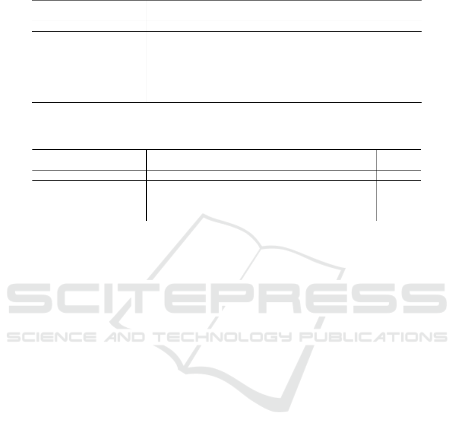
Table 2: MTE on limited subsets of Rotated-MNIST using SF-CNN as baseline (Weiler et al., 2018b).
Number/Percentage of samples
G-Conv II f 500/4.2% 1k/8.3% 2k/17% 4k/33% 6k/50% 12k/100%
x x - 8.635 7.205 5.586 4.684 4.324 3.664 ± 0.082
X x Pooling 3.543 2.529 1.660 1.337 1.126 0.714 ± 0.022
X X Monomials 3.115 2.194 1.593 1.322 1.068 0.677 ± 0.031
X X Global-WS 3.120 2.294 1.614 1.200 1.004 0.712 ± 0.027
X X Local-WS 3.168 2.292 1.612 1.186 1.032 0.688 ± 0.032
X X MLP 3.250 2.310 1.652 1.242 1.024 0.732 ± 0.023
X X MH-SA 3.178 2.268 1.666 1.294 1.038 0.710 ± 0.022
X X SF-II 3.352 2.542 1.836 1.346 1.128 0.782 ± 0.012
E(2)-CNN, Rotation 0.705 ± 0.025
E(2)-CNN, Rotation & Flips 0.682 ± 0.022
Table 3: MTE on limited subsets of SVHN using WRN16-4 (Zagoruyko and Komodakis, 2016) as baseline.
Number/Percentage of samples
G-Conv II f 1k/1.3% 5k/6.9% 10k/14% 50k/69% 73k/100% # Param.
x x - 12.72 6.37 4.96 3.29 3.00 ± 0.01 2.75M
X x Pooling 11.15 5.52 4.46 3.25 2.89 ± 0.09 2.76M
X X Monomials 10.67 5.45 4.51 3.10 2.79 ± 0.03 2.78M
X X Global-WS 11.37 6.45 4.96 3.32 2.95 ± 0.07 2.83M
X X Local-WS 10.70 5.04 4.31 3.00 2.69 ± 0.01 2.77M
sification with limited training data.
We use WRN28-10 and WRN16-8 as baseline ar-
chitecture, respectively and test II with monomials
and local-WS with k = 3. For CIFAR-10, we train on
full data as well as on limited subsets using standard
data augmentation with random crops and flips (Table
4). For STL-10 (Table 5), we use random crops, flips
and cutout (Devries and Taylor, 2017).
On CIFAR-10, we notice two developments:
While our networks outperform the WRN28-10 in the
limited-data domain, indicating an improved sample
complexity, they are unable to achieve better results
in large-data regimes (Table 4). Networks employing
II achieve a better performance than the pooling coun-
terpart among all dataset sizes indicating that II bet-
ter preserves the information needed for a successful
classification leading to a lower sample complexity.
Local-WS performs on par or slightly worse than
the monomials. We conjecture that on bigger dataset
sizes, our approach with its rotation-invariant focus
does not capture the complex local object-related in-
variant cues needed for successful classification as
good as a standard WRN. We remark that for SVHN,
relevant invariance cues besides rotation are rather
global (e.g., color, illumination, noise), while for CI-
FAR these are also local and object-related (e.g., per-
spective changes, occlusions). Thus, our method han-
dles global invariances well while needing additional
steps to handle local invariances other than rotation.
(Weiler and Cesa, 2019) (E(2)-WRN) achieve bet-
ter results than our networks in this setup. However,
their approach differs from ours by loosening equiv-
ariance restrictions with depth and using a bigger in-
variance group including flips, thus addressing more
local invariances. Nevertheless, this approach can be
combined with ours in the future.
On STL-10, both II-enhanced networks outper-
form the equivariant baseline using pooling and the
standard WRN. The local-WS approach outperforms
the monomial counterpart. On this basis, we conclude
that for all practical purposes, II based on local-WS
delivers best results while being simpler to train than
the monomial variant. Again, other methods incorpo-
rating invariance to other groups such as the general
E(2)-CNN (Weiler and Cesa, 2019) or scales (SES-
CNN, (Sosnovik et al., 2020)) achieve better results
than our purely rotation-invariant network. This is
intuitive since samples from ImageNet involve vari-
ability from an even greater source of different trans-
formations than CIFAR-10. Consequently, the invari-
ance cues that need to be captured by a classifier are
even more complex.
6 CONCLUSION
In this contribution, we focused on leveraging prior
knowledge about invariance to transformations for
classification problems. Therefore, we adapted the
II framework by introducing a novel monomial se-
lection algorithm and replacing the monomials with
different functions such as a weighted sum, a MLP,
and self-attention. Replacing the monomials enabled
a streamlined training of DNNs using II by avoiding
the pre-training and selection step. This allows to op-
timally tune and adapt all algorithmic components at
Improving the Sample-complexity of Deep Classification Networks with Invariant Integration
221
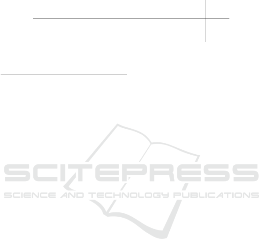
Table 4: MTE on limited subsets of CIFAR-10 using WRN28-10 (Zagoruyko and Komodakis, 2016) as baseline.
Number/Percentage of samples
G-Conv II f 100/0.2% 1k/2% 10k/20% 50k/100% #Param.
x x - 71.69 37.61 9.08 3.89 ± 0.02 36.5M
X x Pooling 76.54 37.29 12.68 4.71 ± 0.04 36.7M
X X Monomials 69.42 29.83 11.15 4.60 ± 0.12 36.8M
X X Local-WS 72.72 32.10 10.45 4.54 ± 0.15 36.9M
E(2)-WRN28-10 2.91 ∼37M
Table 5: MTE on STL-10 using WRN16-8 (Zagoruyko and
Komodakis, 2016) as baseline.
G-Conv II f MTE[%] # Param.
x x - 12.74 ± 0.23 10.97M
X x Pooling 12.51 ± 0.33 10.83M
X X Monomials 10.84 ± 0.46 10.85M
X X Local-WS 10.09 ± 0.21 10.92M
E(2)-WRN16-8 9.80 ± 0.40 12.0M
SES-WRN16-8 8.51 11.0M
once promoting the application of II to complex real-
world datasets and architectures, e.g., WRNs.
Our method explicitly enforces invariance which
we see among the key factors to be taken into consid-
eration by a feature-extraction engine for successful
classification, especially for real-world applications,
where data is often limited. Assuming that rotation
invariance is required, we have shown how to design
a DNN based on II to leverage this prior knowledge.
In comparison to the standard approach, we replace
spatial max-pooling by a dedicated layer which ex-
plicitly enforces invariance while increasing the net-
work’s expressibility. To enable the network to cap-
ture other invariance cues in particular of global na-
ture we use a trainable weights as well.
We have demonstrated state-of-the-art sample
complexity on datasets from various real-world se-
tups. We achieve state-of-the-art results on all data
regimes on image classification tasks when the tar-
geted invariances (i.e., rotation) generate the most in-
traclass variance, as in the case of Rotated-MNIST
and SVHN. On Rotated-MNIST, we even outperform
the E(2)-CNN which also includes invariance to flips.
On CIFAR-10 and STL-10, we show top perfor-
mance in limited-data regimes for image classifica-
tion tasks where various other transformations be-
sides rotation are responsible for the intraclass vari-
ance. At the same time, the performance in the full-
data regime is better than the equivariant baseline,
which shows that we are able to effectively make use
of prior knowledge and introduce rotation invariance
without afflicting other learned invariances. Specifi-
cally, monomials and local-WS achieve the best and
most stable performance and consistently outperform
the baseline, which uses group and spatial pool-
ing, as well as standard convolutional architectures.
Local-WS performs similarly or better than monomi-
als while being easier to apply and optimize due to
avoiding the monomial selection step. It is different to
simply adding an additional group-equivariant layer
and performing average pooling among rotations and
spatial locations because group pooling is performed
before applying the II layer. Compared to TI-Pooling
(Laptev et al., 2016), our method explicitly guaran-
tees invariance within a single forward pass. In con-
trast, TI-Pooling approximates invariance by pooling
among the responses of a non-equivariant network
needing one forward pass per group element.
Our current method is limited to problem settings
where rotation invariance is desired. The expansion to
other transformations is interesting future work. We
also plan to investigate replacing all pooling opera-
tions with II.
ACKNOWLEDGEMENTS
The authors would like to thank their colleagues
Lukas Enderich, Julia Lust and Paul Wimmer for their
valuable contributions and fruitful discussions.
REFERENCES
Bekkers, E. J. (2020). B-spline cnns on lie groups. In ICLR
2020, Addis Ababa, Ethiopia, April 26-30, 2020.
OpenReview.net.
Bekkers, E. J., Lafarge, M. W., Veta, M., Eppenhof, K. A. J.,
Pluim, J. P. W., and Duits, R. (2018). Roto-translation
covariant convolutional networks for medical image
analysis. In MICCAI 2018, Granada, Spain, Septem-
ber 16-20, 2018, Proceedings, Part I, pages 440–448.
Coates, A., Ng, A. Y., and Lee, H. (2011). An analysis of
single-layer networks in unsupervised feature learn-
ing. In Gordon, G. J., Dunson, D. B., and Dud
´
ık, M.,
editors, AISTATS 2011, Fort Lauderdale, USA, April
11-13, 2011, volume 15 of JMLR Proceedings, pages
215–223. JMLR.org.
Cohen, T., Weiler, M., Kicanaoglu, B., and Welling, M.
(2019a). Gauge equivariant convolutional networks
and the icosahedral CNN. In ICML 2019, 9-15 June
2019, Long Beach, CA, USA, pages 1321–1330.
Cohen, T. and Welling, M. (2016). Group equivariant con-
volutional networks. In ICML 2016, New York City,
NY, USA, June 19-24, 2016, pages 2990–2999.
VISAPP 2022 - 17th International Conference on Computer Vision Theory and Applications
222

Cohen, T. S., Geiger, M., and Weiler, M. (2019b). A general
theory of equivariant cnns on homogeneous spaces.
In Wallach, H. M., Larochelle, H., Beygelzimer, A.,
d’Alch
´
e-Buc, F., Fox, E. B., and Garnett, R., editors,
NeurIPS 2019, 8-14 December 2019, Vancouver, BC,
Canada, pages 9142–9153.
Condurache, A. P. and Mertins, A. (2012). Sparse represen-
tations and invariant sequence-feature extraction for
event detection. VISAPP 2012, 1.
Devries, T. and Taylor, G. W. (2017). Improved regular-
ization of convolutional neural networks with cutout.
CoRR, abs/1708.04552.
Diaconu, N. and Worrall, D. E. (2019a). Affine self convo-
lution. CoRR, abs/1911.07704.
Diaconu, N. and Worrall, D. E. (2019b). Learning to con-
volve: A generalized weight-tying approach. In ICML
2019, 9-15 June 2019, Long Beach, California, USA,
pages 1586–1595.
Esteves, C., Allen-Blanchette, C., Makadia, A., and Dani-
ilidis, K. (2018a). Learning SO(3) equivariant repre-
sentations with spherical cnns. In ECCV 2018, Mu-
nich, Germany, September 8-14, 2018, Proceedings,
Part XIII, pages 54–70.
Esteves, C., Allen-Blanchette, C., Zhou, X., and Daniilidis,
K. (2018b). Polar transformer networks. In ICLR
2018.
Falkner, S., Klein, A., and Hutter, F. (2018). BOHB: Robust
and efficient hyperparameter optimization at scale. In
Proceedings of the 35th International Conference on
Machine Learning, pages 1436–1445.
Finzi, M., Welling, M., and Wilson, A. G. (2021). A
practical method for constructing equivariant multi-
layer perceptrons for arbitrary matrix groups. CoRR,
abs/2104.09459.
Freeman, W. T. and Adelson, E. H. (1991). The design
and use of steerable filters. IEEE Trans. Pattern Anal.
Mach. Intell., 13(9):891–906.
Fuchs, F., Worrall, D. E., Fischer, V., and Welling, M.
(2020). Se(3)-transformers: 3d roto-translation equiv-
ariant attention networks. In Larochelle, H., Ranzato,
M., Hadsell, R., Balcan, M., and Lin, H., editors,
NeurIPS 2020, December 6-12, 2020, virtual.
Fuchs, F. B., Wagstaff, E., Dauparas, J., and Posner,
I. (2021). Iterative se(3)-transformers. CoRR,
abs/2102.13419.
Ghosh, R. and Gupta, A. K. (2019). Scale steerable filters
for locally scale-invariant convolutional neural net-
works. CoRR, abs/1906.03861.
Han, S., Pool, J., Tran, J., and Dally, W. J. (2015).
Learning both weights and connections for efficient
neural network. In Cortes, C., Lawrence, N. D.,
Lee, D. D., Sugiyama, M., and Garnett, R., editors,
NeurIPS 2015, December 7-12, 2015, Montreal, Que-
bec, Canada, pages 1135–1143.
Hutchinson, M., Lan, C. L., Zaidi, S., Dupont, E.,
Teh, Y. W., and Kim, H. (2020). Lietransformer:
Equivariant self-attention for lie groups. CoRR,
abs/2012.10885.
Jaderberg, M., Simonyan, K., Zisserman, A., and
Kavukcuoglu, K. (2015). Spatial transformer net-
works. In NeurIPS 2015, pages 2017–2025. Curran
Associates, Inc.
Kanazawa, A., Sharma, A., and Jacobs, D. W. (2014). Lo-
cally scale-invariant convolutional neural networks.
CoRR, abs/1412.5104.
Kingma, D. P. and Ba, J. (2015). Adam: A method for
stochastic optimization. In Bengio, Y. and LeCun, Y.,
editors, ICLR 2015, San Diego, CA, USA, May 7-9,
2015, Conference Track Proceedings.
Kondor, R., Lin, Z., and Trivedi, S. (2018). Clebsch-
gordan nets: a fully fourier space spherical convolu-
tional neural network. In Bengio, S., Wallach, H. M.,
Larochelle, H., Grauman, K., Cesa-Bianchi, N., and
Garnett, R., editors, NeurIPS 2018, 3-8 December
2018, Montr
´
eal, Canada, pages 10138–10147.
Krizhevsky, A. (2009). Learning multiple layers of features
from tiny images,. Technical report.
Laptev, D., Savinov, N., Buhmann, J. M., and Pollefeys, M.
(2016). TI-POOLING: transformation-invariant pool-
ing for feature learning in convolutional neural net-
works. In CVPR 2016, Las Vegas, NV, USA, June 27-
30, 2016, pages 289–297.
Larochelle, H., Erhan, D., Courville, A. C., Bergstra, J.,
and Bengio, Y. (2007). An empirical evaluation of
deep architectures on problems with many factors of
variation. In ICML 2007, Corvallis, Oregon, USA,
June 20-24, 2007, pages 473–480.
LeCun, Y., Bengio, Y., and Hinton, G. E. (2015). Deep
learning. Nature, 521(7553):436–444.
Lee, N., Ajanthan, T., and Torr, P. H. S. (2019). Snip:
single-shot network pruning based on connection sen-
sitivity. In ICLR 2019, New Orleans, LA, USA, May
6-9, 2019. OpenReview.net.
Marcos, D., Kellenberger, B., Lobry, S., and Tuia, D.
(2018). Scale equivariance in cnns with vector fields.
CoRR, abs/1807.11783.
Marcos, D., Volpi, M., Komodakis, N., and Tuia, D. (2017).
Rotation equivariant vector field networks. In ICCV
2017, Venice, Italy, October 22-29, 2017, pages 5058–
5067. IEEE Computer Society.
M
¨
uller, F. and Mertins, A. (2009). Invariant-integration
method for robust feature extraction in speaker-
independent speech recognition. In INTERSPEECH
2009, Brighton, United Kingdom, September 6-10,
2009, pages 2975–2978.
M
¨
uller, F. and Mertins, A. (2010). Invariant integration
features combined with speaker-adaptation methods.
In INTERSPEECH 2010, Makuhari, Chiba, Japan,
September 26-30, 2010, pages 2622–2625.
M
¨
uller, F. and Mertins, A. (2011). Contextual
invariant-integration features for improved speaker-
independent speech recognition. Speech Communica-
tion, 53(6):830–841.
Netzer, Y., Wang, T., Coates, A., Bissacco, A., Wu, B., and
Ng, A. Y. (2011). Reading digits in natural images
with unsupervised feature learning. NIPS Workshop
on Deep Learning and Unsupervised Feature Learn-
ing.
Noether, E. (1916). Der endlichkeitssatz der invarianten
endlicher gruppen. Mathematische Annalen, 77:89–
92.
Improving the Sample-complexity of Deep Classification Networks with Invariant Integration
223

Rath, M. and Condurache, A. P. (2020). Invariant integra-
tion in deep convolutional feature space. In ESANN
2020, Bruges, Belgium, October 2-4, 2020, pages
103–108.
Reisert, M. and Burkhardt, H. (2006). Invariant features
for 3d-data based on group integration using direc-
tional information and spherical harmonic expansion.
In ICPR 2006, 20-24 August 2006, Hong Kong, China,
pages 206–209. IEEE Computer Society.
Romero, D. W., Bekkers, E. J., Tomczak, J. M., and
Hoogendoorn, M. (2020). Attentive group equivariant
convolutional networks. In ICML 2020, 13-18 July
2020, Virtual Event, pages 8188–8199. PMLR.
Romero, D. W. and Cordonnier, J. (2020). Group equiv-
ariant stand-alone self-attention for vision. CoRR,
abs/2010.00977.
Romero, D. W. and Hoogendoorn, M. (2020). Co-attentive
equivariant neural networks: Focusing equivariance
on transformations co-occurring in data. In ICLR
2020, Addis Ababa, Ethiopia, April 26-30, 2020.
OpenReview.net.
Schulz-Mirbach, H. (1992). On the existence of complete
invariant feature spaces in pattern recognition. In Pat-
tern Recognition: Eleventh International Conference
1992, pages 178 – 182.
Schulz-Mirbach, H. (1994). Algorithms for the construction
of invariant features. In Tagungsband Mustererken-
nung 1994 (16. DAGM Symposium), Reihe Informatik
Xpress, Nr.5, pages 324–332.
Schulz-Mirbach, H. (1995). Invariant features for gray
scale images. In Mustererkennung 1995, 17. DAGM-
Symposium, Bielefeld, 13.-15. September 1995, Pro-
ceedings, pages 1–14.
Shaw, P., Uszkoreit, J., and Vaswani, A. (2018). Self-
attention with relative position representations. In
Walker, M. A., Ji, H., and Stent, A., editors, NAACL-
HLT 2018, New Orleans, Louisiana, USA, June 1-6,
2018, Volume 2 (Short Papers), pages 464–468. Asso-
ciation for Computational Linguistics.
Sosnovik, I., Szmaja, M., and Smeulders, A. W. M. (2020).
Scale-equivariant steerable networks. In ICLR 2020,
Addis Ababa, Ethiopia, April 26-30, 2020.
Tai, K. S., Bailis, P., and Valiant, G. (2019). Equivariant
transformer networks. In ICML 2019, 9-15 June 2019,
Long Beach, California, USA, pages 6086–6095.
Veeling, B. S., Linmans, J., Winkens, J., Cohen, T., and
Welling, M. (2018). Rotation equivariant CNNs for
digital pathology. CoRR, abs/1806.03962.
Walters, R., Li, J., and Yu, R. (2020). Trajectory predic-
tion using equivariant continuous convolution. CoRR,
abs/2010.11344.
Weiler, M. and Cesa, G. (2019). General e(2)-equivariant
steerable cnns. In NeurIPS 2019, 8-14 December
2019, Vancouver, BC, Canada, pages 14334–14345.
Weiler, M., Geiger, M., Welling, M., Boomsma, W., and
Cohen, T. (2018a). 3d steerable cnns: Learning ro-
tationally equivariant features in volumetric data. In
Bengio, S., Wallach, H. M., Larochelle, H., Grau-
man, K., Cesa-Bianchi, N., and Garnett, R., edi-
tors, NeurIPS 2018, 3-8 December 2018, Montr
´
eal,
Canada, pages 10402–10413.
Weiler, M., Hamprecht, F. A., and Storath, M. (2018b).
Learning steerable filters for rotation equivariant cnns.
In CVPR 2018, Salt Lake City, UT, USA, June 18-22,
2018, pages 849–858.
Winkels, M. and Cohen, T. S. (2019). Pulmonary nodule
detection in CT scans with equivariant cnns. Medical
Image Anal., 55:15–26.
Worrall, D. E. and Brostow, G. J. (2018). Cubenet: Equiv-
ariance to 3d rotation and translation. In ECCV 2018,
Munich, Germany, September 8-14, 2018, Proceed-
ings, Part V, pages 585–602.
Worrall, D. E., Garbin, S. J., Turmukhambetov, D., and
Brostow, G. J. (2017). Harmonic networks: Deep
translation and rotation equivariance. In 2017 IEEE
Conference on Computer Vision and Pattern Recog-
nition, CVPR 2017, Honolulu, HI, USA, July 21-26,
2017, pages 7168–7177.
Worrall, D. E. and Welling, M. (2019). Deep scale-spaces:
Equivariance over scale. In NeurIPS 2019, 8-14 De-
cember 2019, Vancouver, BC, Canada, pages 7364–
7376.
Xu, Y., Xiao, T., Zhang, J., Yang, K., and Zhang, Z. (2014).
Scale-invariant convolutional neural networks. CoRR,
abs/1411.6369.
Yang, F., Wang, Z., and Heinze-Deml, C. (2019).
Invariance-inducing regularization using worst-case
transformations suffices to boost accuracy and spatial
robustness. In NeurIPS 2019, 8-14 December 2019,
Vancouver, BC, Canada, pages 14757–14768.
Zagoruyko, S. and Komodakis, N. (2016). Wide resid-
ual networks. In Wilson, R. C., Hancock, E. R.,
and Smith, W. A. P., editors, BMVC 2016, York, UK,
September 19-22, 2016. BMVA Press.
Zhu, W., Qiu, Q., Calderbank, A. R., Sapiro, G., and
Cheng, X. (2019). Scale-equivariant neural net-
works with decomposed convolutional filters. CoRR,
abs/1909.11193.
APPENDIX
Implementation Details. To increase the repro-
ducibility, we provide our exact hyper-parameter set-
tings. We optimized the standard Wide-ResNets using
stochastic gradient descent and the hyper-parameters
of the corresponding paper (Zagoruyko and Ko-
modakis, 2016). All steerable networks were op-
timized using Adam optimization (Kingma and Ba,
2015). We used exponential learning rate decay
for Rotated-MNIST and SVHN, while we employed
step-wise decay on CIFAR-10 and STL-10. All steer-
able filter weights were regularized using elastic net
regularization with factor 10
−7
(cf. (Weiler et al.,
2018b)). For all WRNs, we additionally use `
2
-
regularization for the learnable BatchNorm coeffi-
cients with factor 0.1. All regularization losses were
then multiplied by the regularization constant.
VISAPP 2022 - 17th International Conference on Computer Vision Theory and Applications
224

Table 6: II-SF-CNN hyper-parameters on Rotated-MNIST.
Hyper-parameter MH-SA Global-WS Local-WS MLP SF-Conv Monomials SF-CNN
Optimizer Adam Adam Adam Adam Adam Adam Adam
Batch Size 32 32 32 32 32 32 64
Epochs 100 100 100 100 100 100 100
n
FC
95 85 30 85 85 90 96
Learning Rate 5e-3 1e-4 1e-3 1e-4 5e-4 1e-4 1e-3
LR Decay 0.5 0.1 0.5 0.1 0.2 0.75 0.9
LR Decay Epoch 20 40 25 30 25 15 20
Reg. Constant 1e-3 0.1 1e-3 1e-3 0.01 0.15 1.
Dropout Rate 0.05 0.45 0.4 0.5 0.4 0.45 0.7
Attention Heads 1 - - - - - -
Attention Dropout 0. - - - - - -
Table 7: Hyper-parameters on SVHN.
Hyper-parameter SF-CNN Global-WS Local-WS Monomials
Optimizer Adam Adam Adam Adam
Batch Size 128 128 128 64
Epochs 100 100 100 100
n
FC
32 64 36 85
Learning Rate 1e-3 5e-4 5e-4 5e-4
LR Decay 0.4 0.1 0.25 0.25
LR Decay Epoch 20 30 25 20
Reg. Constant 2e-3 0.25 0.2 0.05
Dropout Rate 0.55 0.7 0.5 0.7
Table 8: Hyper-parameters on CIFAR-10.
Hyper-parameter SF-CNN Local-WS Monomials
Optimizer Adam Adam Adam
Batch Size 64 64 64
Epochs 100 100 100
n
FC
- 90 30
Learning Rate 1e-3 5e-4 5e-4
LR Decay 0.5 0.2 0.025
LR Decay Epoch 50 50 50
Reg. Constant 0.1 5e-6 0.008
Dropout Rate 0.3 0.1 0.4
Table 9: Hyper-parameters on STL-10.
Hyper-parameter SF-CNN Local-WS Monomials
Optimizer Adam Adam Adam
Batch Size 96 64 32
Epochs 1000 1000 1000
n
FC
- 16 10
Learning Rate 5e-4 0.01 5e-4
LR Decay 0.1 0.3 0.1
LR Decay Epoch 300 300 300
Reg. Constant 1e-8 1e-9 5e-9
Dropout Rate 0.1 0.15 0.05
The hyper-parameters were optimized using
Bayesian Optimization with Hyperband (BOHB,
(Falkner et al., 2018)) on 80/20 validation splits, if
it was not already predetermined by the dataset. They
are shown in Tables 6-9. On Rotated-MNIST we used
data augmentation with random rotations following
(Weiler et al., 2018b). On CIFAR-10 and SVHN, we
followed (Zagoruyko and Komodakis, 2016) and used
random crops and flips for CIFAR-10 and no data
augmentation for SVHN. On STL-10, we use random
crops, flips and cutout (Devries and Taylor, 2017) .
For the monomial architectures, we applied II per
channel, and pruned M = 50 initial monomials to
n
m
= 5 for Rot-MNIST and n
m
= 10 monomials for
SVHN, CIFAR-10 and STL-10. We used one inter-
mediate pruning step after 10 epochs with n
m
= 25
and train additional 5 epochs before the final pruning
step. All other invariant integration layers were im-
plemented with constant number of channels.
Number of Parameters. For our invariant architec-
tures, we keep the number of parameters constant by
reducing the number of channels accordingly. A stan-
dard convolutional filter with kernel size k, c
i
input
channels and c
o
output channels has k
2
c
i
c
o
parame-
ters. A rotation-steerable filter has 2n
F
n
α
c
i
c
o
param-
eters with n
α
rotations and n
F
basis filters. In order to
keep the number of parameters constant, we equate
k
2
c
i
c
o
= 2n
F
n
α
˜c
i
˜c
o
⇔
˜c
i
˜c
o
c
i
c
o
=
2n
F
n
α
k
2
(16)
We use k = 3, n
α
= 8, n
F
= 16 and obtain a final ratio
of
256
9
by which we need to reduce c
i
c
o
. Hence, we
reduce the number of channels by
q
256
9
=
16
3
. For
the lifting convolution, the filter is not used among all
rotations, so we only need to reduce the ratio by
q
32
9
.
Improving the Sample-complexity of Deep Classification Networks with Invariant Integration
225
