An Activation Function with Probabilistic Beltrami Coefficient for

Deep Learning

Hirokazu Shimauchi

Hachinohe Institute of Technology, Hachinohe, Aomori, Japan

Keywords: Activation Function, Neural Network, Beltrami Coefficient, Quasiconformal Mapping, Stochastic

Perturbation.

Abstract: We propose an activation function that has a probabilistic Beltrami coefficient for deep neural networks.

Activation functions play a crucial role in the performance and training dynamics of deep learning models. In

recent years, it has been suggested that the performance of real-valued neural networks can be improved by

adding a stochastic perturbation term to the activation function. Meanwhile, numerous studies have been

conducted on activation functions of complex-valued neural networks. The proposed approach

probabilistically deforms the Beltrami coefficient of complex-valued activation functions. The Beltrami

coefficient represents the distortion by mapping at each point. In previous research, when dealing with

complex numbers, adding a perturbation term meant applying probabilistic parallel translation from a

geometric viewpoint. By contrast, our approach introduces a stochastic perturbation for rotation and scaling.

Our experimental results show that the proposed activation function improves the performance of image

classification tasks, implying that the suggested activation function produces effective representations during

training.

1 INTRODUCTION

We propose an activation function for deep complex-

valued neural networks that have probabilistic

Beltrami coefficients. In this section, we summarise

the background, related works, and contributions of

this study.

1.1 Background and Related Works

Activation functions introduce nonlinearity to neural

networks, which helps in obtaining a complex

representation of data; the choice of these functions

significantly affects the performance of deep learning

models (Karlik and Olgac, 2011). Therefore,

activation functions have been widely researched.

1.1.1 Deterministic Real-valued Activation

Functions

In the early days, sigmoid and tanh (hyperbolic

tangent) activation functions were widely used

(Schmidhuber, 2015). However, these became

https://orcid.org/0000-0002-9160-5667

ineffective in deep neural networks because of the

vanishing gradient problem. The rectified linear unit

(ReLU) (Nair and Hinton, 2010), a piecewise linear

activation function, showed better generalisation

performance in deep learning compared with

sigmoid and tanh. However, there are some well-

known weaknesses of ReLU. One of them is called

the dying ReLU, which is related to a gradient

information loss caused by the collapse of the

negative inputs to zero. Therefore, numerous

activation functions have been developed to

improve performance and address the shortcomings

of ReLU, such as leaky ReLU (Xu et al. 2015),

parametric ReLU (PreLU) (He et al., 2015),

exponential linear unit (ELU) (Clevert, 2015),

scaled exponential linear unit (SELU) (Klambauer

et al., 2017), sigmoid-weighted linear unit (Swish)

(Ramachandran et al., 2017), and Mish (Misra,

2019). These are deterministic functions with fixed

input–output relationships.

Shimauchi, H.

An Activation Function with Probabilistic Beltrami Coefﬁcient for Deep Learning.

DOI: 10.5220/0010870500003116

In Proceedings of the 14th International Conference on Agents and Artiﬁcial Intelligence (ICAART 2022) - Volume 3, pages 613-620

ISBN: 978-989-758-547-0; ISSN: 2184-433X

613

1.1.2 Probabilistic Real-valued Activation

Functions

Recently, Shridhar et al. (2019) proposed ProbAct, a

probabilistic activation function, which is inspired by

the stochastic behaviour of biological neurones.

Uncertain biomechanical effects may cause noise in

neuronal spikes (Lewicki, 1998). Shridhar et al.

(2019) aimed to emulate a similar behaviour in the

information flow to the neurones by adding stochastic

perturbation terms with trainable or nontrainable

weights. It was shown that ProbAct improves the

performance of various visual and textual

classification tasks. In particular, they confirmed that

the augmentation-like operation in ProbAct was

effective even when there are a few data points.

1.1.3 Deterministic Complex-valued

Activation Functions

In parallel with the studies on real-valued cases,

research on complex-valued activation functions for

deep complex-valued neural networks has been

conducted. Liouville’s theorem states that the only

complex-analytic and bounded function is a constant

function. The construction of the analytic activation

function is a challenging task in the complex case.

However, Hirose and Yoshida (2012) showed that

limiting the regularity of the activation functions to

only analytic functions is unnecessarily restrictive.

Recently, numerous complex activations inspired by

ReLU have been proposed, for example, zReLU

(Guberman, 2016), modReLU (Arjovsky et al.,

2016), and CReLU (Xu et al., 2015). CReLU is a

complex function that applies separate ReLUs on

both the real and imaginary parts of a neuron; it

outperforms both modReLU and zReLU in the

experiments in CIFAR 10 and CIFAR 100

(Krizhevsky et al., 2009).

1.2 Contributions of This Study

We propose a complex-valued activation function,

BelAct, which has probabilistic Beltrami coefficients.

Our experiments show that the proposed activation

function shows better accuracy on benchmark

datasets compared with baseline models. In

particular, the combination of ProbAct and BelAct

increases performance when there are a few data

points, and hence, BelAct may produce essentially

different useful representations of features compared

with ProbAct. The remainder of this paper is

organised as follows.

In the next section, we propose BelAct and

consider the geometric meaning of this operation

from the viewpoint of complex functions. The

evaluation of the proposed activation function for

image classification tasks is presented in Section 3. In

the last section, we conclude the paper and propose

directions for future work.

2 ACTIVATION FUNCTION

WITH PROBABILISTIC

BELTRAMI COEFFICIENT

In this section, we define BelAct and ProbBelAct

using probabilistic quasiconformal linear mappings.

2.1 Quasiconformal Mapping and

Beltrami Coefficient

Let 𝐷 and 𝐷′ be the domains in the complex plane. A

sense-preserving homeomorphism

𝑓: 𝐷 → 𝐷′is

called

a quasiconformal mapping if 𝑓 satisfies the following

two properties:

 For any closed rectangle 𝑅 in 𝐷, f is absolutely

continuous on almost every horizontal and

vertical line in

𝑅.

 There exists a real number

𝐾>1, and the

dilatation condition

𝑓



(𝑧)| ≤

𝐾−1

𝐾+1

𝑓



(𝑧)

(1)

holds almost everywhere in D.

Quasiconformal mappings play important roles in

various fields, such as complex dynamical systems

and the Teichmüller theory in the fields of

mathematics (see Ahlfors, 2006 for details) and

image processing in the medical field.

The complex function

𝜇

(

𝑧

)

𝑓



(𝑧)

𝑓



(𝑧)

(2)

where

𝑓



:=(

𝑓



−𝑖

𝑓



)/2

(3)

and

𝑓



:=(

𝑓



+𝑖

𝑓



)/2,

(4)

is defined on almost everywhere for a quasiconformal

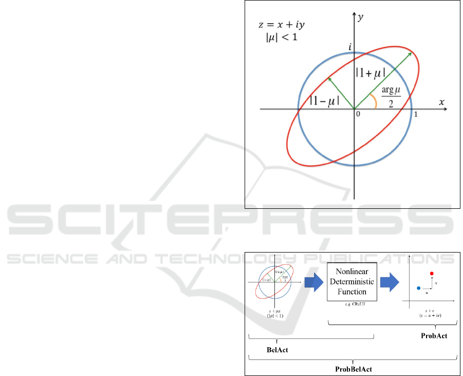
mapping 𝑓, and is called the Beltrami coefficient. The

Beltrami coefficient represents the distortion of

mapping at each point (see function ℎ



in Section 2.4

and Figure 1 for an example).

ICAART 2022 - 14th International Conference on Agents and Artiﬁcial Intelligence

614

2.2 Definition of BelAct

We define an activation function called BelAct as

𝑓

(𝑧) ≔ 𝑔(𝑧 + 𝑠



𝜇𝑧

), (5)

where 𝑧 is the real or complex number input and 𝑔 is

a fixed activation function (for example, 𝑔

(

𝑧

)

max

(

0, 𝑥

)

+𝑖max

(

0, 𝑦

)

, where 𝑧=𝑥+𝑖𝑦 is

CReLU). The perturbation parameter 𝑠



is a fixed or

trainable value, which specifies the range of

stochastic perturbation, and 𝜇 is a random value

sampled from the real and imaginary parts from a

normal distribution 𝑁(0; 1) . We call 𝑔 the base

function of BelAct.

2.3 Definition of ProbBelAct

The ProbAct (Shridhar et al., 2019) is defined as

𝑓

(

𝑧

)

≔𝑔

(

𝑧

)

+𝑠



𝑒, (6)

where 𝑠



is a fixed or trainable value that specifies the

range of stochastic perturbation, and 𝑒 is a random

value. Considering the complex case, adding a

perturbation term like ProbAct geometrically means

probabilistic parallel translation. By contrast, BelAct

adds probabilistic rotation and scaling to the input via

probabilistic quasiconformal linear mappings. The

combination of ProbAct and BelAct (we call it

ProbBelAct) can be considered as

𝑓

(

𝑧

)

≔𝑔

(

𝑧+𝑠



𝜇𝑧

)

+𝑠



𝑒.

(7)

2.4 Geometric Meaning of ProbAct and

BelAct

We consider the mapping

ℎ



(

𝑧

)

≔𝑧+𝑐

(8)

and

ℎ



(

𝑧

)

≔𝑧+𝜇𝑧

(9)

where 𝑐 and 𝜇 are complex constants. When 𝑐=𝑢+

𝑖𝑣 with 𝑢 and 𝑣 as real numbers and 𝑖 is an imaginary

number, ℎ



moves the input 𝑢 in the

𝑥-axis direction

and 𝑣 in the 𝑦-axis direction. Thus, ProbAct can be

considered as adding a parallel translation to the

output of 𝑔.

ℎ



rotates and scales the input depending on 𝜇, as

shown in Figure 1, on the whole complex plane.

Therefore, BelAct adds rotation and scaling to the

input. In general, the Beltrami coefficients of a

quasiconformal mapping

𝑓 are defined as equation

(2) in Section 2.1. 𝜇(𝑧) describes how 𝑓 deforms the

neighbourhoods of each point, compared with

conformal mapping; recall that conformal mapping is

an injective and analytic function that preserves the

local geometry. ℎ



can be considered as a conformal

linear mapping, and its Beltrami coefficient is zero

everywhere. ℎ



is a quasiconformal linear mapping

with a constant Beltrami coefficient 𝜇. An overview

of the ProbAct (right), BelAct (left), and ProbBelAct

is presented in Figure 2.

Figure 1: Distortion by a quasiconformal linear mapping ℎ



that has Beltrami coefficient 𝜇.

Figure 2: Overview of ProbAct, BelAct, and ProbBelAct on

the complex plane.

2.5 Setting the Base Function and the

Parameter for Stochastic

Perturbations

We chose CReLU as the base function for BelAct and

ProbBelAct in our experiments. Regarding the

parameter for stochastic perturbation 𝑠



of the

Beltrami coefficient 𝜇 for BelAct, we consider two

cases like setting 𝑠



of ProbAct (Shridhar et al. 2019):

fixed and trainable. 𝜇 of BelAct represents how far

An Activation Function with Probabilistic Beltrami Coefﬁcient for Deep Learning

615

from the conformal mapping the image is: if |𝜇| i s

large, the image is deformed strongly by ℎ



. In

particular, if

𝜇

=1, the image is degenerated to a

line when ℎ



is applied. Hence, it is natural that we

restrict

𝑠



𝜇

<1 . This setting means that ℎ



preserves the orientation and is an injective mapping.

2.5.1 Fixed Case

For the fixed case, 𝑠



is a constant hyperparameter.

This can be viewed as a repeated perturbation of the

scaled Gaussian noise to the Beltrami coefficients.

Herein, we set 𝑠



=𝑠



=0.05 by considering that

the data are normalised by the standardisation in our

experiments.

2.5.2 Trainable Case

For the trainable case, we treat 𝑠



as a trainable

parameter, which reduces the requirement to

determine 𝑠



as a hyperparameter. Here, we consider

two settings for trainable cases. One of the settings is

a shared trainable 𝑠



across the network. In this case,

a single extra parameter used for all the BelAct layers

was introduced. In the other case, a trainable

parameter is introduced for each input element. In all

cases, the complex network is optimised using a

gradient-based algorithm such as an adaptive moment

estimation (Adam).

3 EXPERIMENTS

In this section, we present the empirical evaluations

of the BelAct and ProbAct in image classification

tasks.

3.1 Dataset

We use the CIFAR 10 and CIFAR 100 datasets. All

inputs were normalised using standardisation.

Furthermore, we also verify the performance of these

activation functions when the number of training data

is reduced because the ProbAct as reported by

Shridhar et al. (2019) is effective even when the

number of data points is less.

3.2 Experimental Settings

To evaluate the performance of the proposed

activation function, we compared it to the following

activation functions: ReLU, Sigmoid, Tanh, SELU,

and Swish for the real-valued neural network, and

CReLU, ProbAct with CReLU for the complex-

valued neural network. The selected deterministic

activation functions are widely used. These are

suitable as baselines.

Table 1: List of hyperparameters.

aramete

Value

Kernel size for

convolution

Padding Same

Kernel size for max-

ooling

Max-

ooling stride 2

timize

Adam

Batch size 128

Learning rate 0.0001

(0.00001 after 50 epochs)

Number of e

ochs 100

Fixed s

, s

0.05

Single trainable

initialise

Element-wise trainable

initialise

Xavier initialisation

3.2.1 Architecture of the Neural Network

We chose a simple architecture, specific hyper-

parameters, and training settings to compare the

performance of the activation functions. We utilised

a VGG16 neural network architecture for image

classification tasks (Simonyan and Zisserman, 2014).

The architecture used in the experiments is defined as

64, 64, M, 128, 128, M, 256, 256, 256, M, 512, 512,

512, M, 512, 512, 512, M, FC, and FC, where

numbers represent the filters of a two-dimensional

real or complex convolution layer, which are

followed by an activation function. M represents the

max-pooling layer, and FC represents the fully

connected layer with 4,096 units. After the last layer

of the real-valued case, the softmax activation is used

with 10 and 100 units for CIFAR 10 and CIFAR 100,

respectively. The softmax real with the average

function in (Barrachina, 2019) was used for the

complex-valued case. The detailed settings are

presented in Table 1. Regularisation tricks, pre-

training, dropout, and batch normalisation are

avoided in this experiment for the comparison of

activation functions.

3.2.2 Implementation

For the implementation, we used Python 3.7.9, with

Tensorflow 2.5.0. Further, the Complex-Valued

Neural Networks (CVNN) (Barrachina 2019) library

is also used for the complex-valued neural networks.

BelAct and ProbBelAct can simply be implemented

ICAART 2022 - 14th International Conference on Agents and Artiﬁcial Intelligence

616

as a function (fixed case) or a custom layer (trainable

cases) of Keras in Tensorflow.

3.3 Results on CIFAR 10

The CIFAR-10 dataset consists of 60,000 images

with 32 × 32 pixels for each image. It has 10 classes

with 6,000 images per class and is split into 50,000

training images and 10,000 test images. The training

data are augmented by the image generator of Keras

during training. We used the accuracy on the test

dataset for the comparison. All experiments were

performed three times, and the reported values are the

average of the three. The results for the CIFAR 10 are

presented in Table 2. The average score in three

independent trials was used as the final evaluation

metric.

Table 2: Results on CIFAR 10 (average of three trials).

Activation Function Accurac

ReLU 0.845

sigmoi

0.100

Tanh 0.833

SeLU 0.857

Swish 0.859

CReLU 0.864

ProbAct (fixed) 0.866

ProbAct (single trainable) 0.866

ProbAct (element wise trainable) 0.867

BelAct

(

fixed

)

0.870

BelAct

(

sin

le trainable

)

0.870

BelAct

(

element wise trainable

)

0.868

ProbBelAct (fixed) 0.866

ProbBelAct (single trainable) 0.869

ProbBelAct (element-wise

trainable

)

0.868

BelAct with the fixed scalar and single trainable

cases achieved the best score. In this experiment, the

score improved by 2.5% compared to the case of

ReLU. In addition, the other cases of BelAct and

ProbBelAct improve the score by 2.1%–2.4%.

However, the difference between the best score and

the CReLU was 0.6%.

3.4 Results on CIFAR 100

There are 100 classes with 600 images with 32 × 32

pixels for each image per class in the CIFAR-100

dataset. Therefore, the number of training data per

class was only 10% for CIFAR10. As in the case of

CIFAR 10, we split the dataset into 50,000 training

images and 10,000 test images and used accuracy on

the test dataset for this experiment.

Table 3 shows the results for the CIFAR 100. In

this case, the best score was achieved by the

ProbBelAct with a fixed scaling parameter. When

using the ProbBelAct with a fixed parameter, we

achieved performance improvements of 3.6% and

1.6% compared to ReLU and CReLU, respectively.

Table 3: Results on CIFAR 100 (average of three trials).

Activation Function Accurac

ReLU 0.513

moi

0.010

Tanh 0.508

SeLU 0.517

Swish 0.520

CReLU 0.534

ProbAct

(

fixed

)

0.531

ProbAct (single trainable) 0.534

ProbAct (element wise trainable) 0.535

BelAct (fixed) 0.541

BelAct

(

sin

le trainable

)

0.539

BelAct

(

element-wise trainable

)

0.536

ProbBelAct

(

fixed

)

0.549

ProbBelAct (single trainable) 0.535

ProbBelAct (element-wise trainable) 0.538

3.5 Results on Reduced CIFAR 10

In Sections 3.2.2 and 3.2.3, the performance of

BelAct and ProbBelAct showed high performance on

CIFAR 10 and CIFAR 100. Motivated by the

augmentation property of ProbAct, we further

verified the performance when the training dataset

was reduced. Here, the ratio of training data and test

data is swapped. We split the dataset into 10,000

training images and 60,000 test images. The results of

the reduced CIFAR 10 are shown in Table 4.

Table 4: Results on reduced CIFAR 10 (average of three

trials).

Activation Function Accurac

ReLU 0.683

CReLU 0.708

ProbAct

(

fixed

)

0.706

ProbAct

(

sin

le trainable

)

0.711

ProbAct

(

element-wise trainable

)

0.713

BelAct (fixed) 0.711

BelAct (single trainable) 0.704

BelAct (element-wise trainable) 0.714

ProbBelAct

(

fixed

)

0.708

ProbBelAct

(

sin

le trainable

)

0.706

ProbBelAct (element-wise trainable) 0.709

The best score was achieved by the BelAct with

element-wise trainable scaling parameters. There

An Activation Function with Probabilistic Beltrami Coefﬁcient for Deep Learning

617

were 3.1% and 0.6% improvements over the case of

ReLU and CReLU, respectively.

Table 5: Results on reduced CIFAR 100 (average of three

trials).

Activation Function Accurac

ReLU 0.277

CReLU 0.285

ProbAct (fixed) 0.290

ProbAct (single

trainable

)

0.289

ProbAct (element-wise

trainable

)

0.289

BelAct

(

fixed

)

0.285

BelAct (single trainable) 0.284

BelAct (element wise

trainable

)

0.281

ProbBelAct

(

fixed

)

0.287

ProbBelAct (single

trainable

)

0.292

ProbBelAct (element-

wise trainable)

0.278

3.6 Results on Reduced CIFAR 100

A similar experiment as described in Section 3.5 was

also performed for CIFAR 100. The CIFAR 100

dataset was split into 10,000 training images and

60,000 test images. Table 5 shows the results for the

reduced CIFAR 100. When using the ProbBelAct

with a single trainable parameter, we achieved the

best performance in this case. The scores increased by

1.5% and 0.7% compared to ReLU and CReLU,

respectively.

4 DISCUSSION

In Section 3.3 and 3.4, it is observed that the

improved score on CIFAR 100 is larger than that of

CIFAR 10. It has been proposed that ProbAct can be

considered an augmentation operation (Shridhar et

al., 2019). BelAct is also viewed as an augmentation

technique; however, the operation is essentially

different from that of ProbAct (see Section 2).

ProbBelAct achieved the best score in the cases of

CIFAR 100 (original case and reduced case), and it

should be noted that the size of training data per class

of CIFAR 100 is ten per cent of the case of CIFAR

10. It could be suggested that ProbBelAct further

extends the diversity of representation space

compared to the ProbAct.

There are other methods for training neural

networks which use random distributions. One well-

known method is the dropout layer, which generalises

by vanishing the units at random during training and

can be interpreted as a model ensemble method.

Moreover, several studies on the effects of adding

noise to weights, inputs, and gradients have been

conducted. Conversely, the BelAct and ProbBelAct

follow the concept proposed by Bengio et al. (2013),

like ProbAct: stochastic neurones with sparse

representations allow internal regularisation.

5 CONCLUSIONS

We proposed a novel activation function that has a

probabilistic Beltrami coefficient, called BelAct.

Adding the operation of ProbAct, ProbBelAct was

also presented. The proposed activation function

shows better performance compared with the baseline

models on both CIFAR 10 and CIFAR 100 datasets.

In particular, ProbBelAct achieved the best score

on the CIFAR 100 dataset. It could be suggested that

ProbBelAct brings a richer representation of features

compared with ProbAct and BelAct on small datasets.

In future, we intend to apply our method to smaller

image classification tasks. Furthermore, we will

verify the effectiveness of BelAct and ProbBelAct in

natural language processing tasks.

ACKNOWLEDGEMENTS

We would like to thank the reviewers for their time

spent reviewing our manuscript. This work was

supported by JSPS KAKENHI (Grant Number

20K23330).

REFERENCES

Ahlfors, L.V. (2006). Lectures on quasiconformal

mappings: second edition, University Lecture Series,

Vol. 38, American Mathematical Society, Providence.

Arjovsky, M., Shah, A., Bengio, Y. (2016). Unitary

evolution recurrent neural networks. arXiv preprint

arXiv:1511.06464.

Barrachina, J. A. (2019). Complex-valued neural networks

(CVNN), Available: https://github.com/NEGU93/cvnn.

Bengio, Y., Léonard, N., Courville, A. (2013). Estimating

or propagating gradients stochastic neurons for

conditional computation. arXiv preprint

arXiv:1308.3432.

Clevert, D.-A., Unterthiner, T., Hochreiter, S. (2015). Fast

and accurate deep network learning by exponential

linear units (elus). arXiv preprint arXiv:1511.07289.

Guberman, N. (2016). On complex valued convolutional

neural networks. arXiv preprint arXiv:1602.09046.

ICAART 2022 - 14th International Conference on Agents and Artiﬁcial Intelligence

618

He, K., et al. (2015). Delving deep into rectifiers:

Surpassing human-level performance on imagenet

classification. In Proceedings of the 2015 IEEE

International Conference on Computer Vision.

Hirose, A., Yoshida, S. (2012). Generalization

characteristics of complex-valued feedforward neural

networks in relation to signal coherence. IEEE

Transactions on Neural Networks and Learning

Systems 23.4, 541-551.

Karlik, B., Vehbi Olgac, A. (2011). Performance analysis

of various activation functions in generalized MLP

architectures of neural networks. International Journal

of Artificial Intelligence and Expert Systems 1.4, 111-

122.

Klambauer, G., et al. (2017). Self-normalizing neural

networks. In Proceedings of the 31st International

Conference on Neural Information Processing Systems.

Krizhevsky, A., Nair, V., Hinton, G. Cifar-10 (Canadian

Institute for Advanced Research), Available:

http://www.cs.toronto.edu/~kriz/cifar.html

Lewicki, M.S. (1998). A review of methods for spike

sorting: the detection and classification of neural action

potentials. Network: Computation in Neural Systems

9.4, R53.

Misra, D. (2019). Mish: A self regularized non-monotonic

neural activation function. arXiv preprint

arXiv:1908.08681.

Nair, V., Hinton, G.E. (2010). Rectified linear units

improve restricted Boltzmann machines. In

Proceedings of the International Conference on

Machine Learning 2010, 807–814.

Ramachandran, P., Zoph, B., Le, Q.V. (2017). Searching

for activation functions. arXiv preprint

arXiv:1710.05941.

Schmidhuber, J. (2015). Deep learning in neural networks:

An overview. Neural networks 61, 85-117.

Shridhar, K., et al. (2019). ProbAct: A probabilistic

activation function for deep neural networks. arXiv

preprint arXiv:1905.10761.

Simonyan, K., Zisserman, A. (2014). Very deep

convolutional networks for large-scale image

recognition. arXiv preprint arXiv:1409.1556.

Trabelsi, C., et al. (2017). Deep complex networks. arXiv

preprint arXiv:1705.09792.

Xu, B., et al. (2015). Empirical evaluation of rectified

activations in convolutional network. arXiv preprint

arXiv:1505.00853.

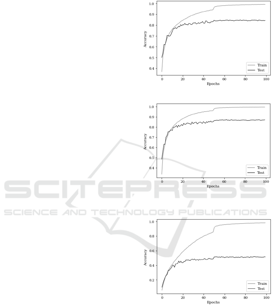
APPENDIX

Here, we show the learning curves of ReLU and the

activation function that attained the highest score on

CIFAR 10, CIFAR 100, reduced CIFAR 10, and

reduced CIFAR 100.

Figure 3: Learning curve of ReLU on CIFAR 10.

Figure 4: Learning curve of the activation function that

attained the highest score on CIFAR 10 (BelAct with a

single trainable parameter).

Figure 5: Learning curve of ReLU on CIFAR 100.

An Activation Function with Probabilistic Beltrami Coefﬁcient for Deep Learning

619

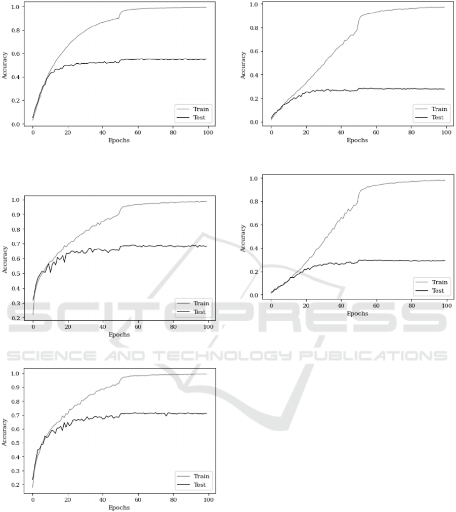
Figure 6: Learning curve of the activation function that

attained the highest score on CIFAR 100 (ProbBelAct with

fixed parameter).

Figure 7: Learning curve of ReLU on reduced CIFAR 10.

Figure 8: Learning curve of the activation function that

attained the highest score on reduced CIFAR 10 (BelAct

with an element-wise trainable parameter).

Figure 9: Learning curve of ReLU on reduced CIFAR 100.

Figure 10: Learning curve of the activation function that

attained the highest score on reduced CIFAR 100

(ProbBelAct with a single trainable parameter).

ICAART 2022 - 14th International Conference on Agents and Artiﬁcial Intelligence

620