Tackling Train Routing via Multi-agent Pathﬁnding and

Constraint-based Scheduling

svancara

and Roman Bart

Charles University, Faculty of Mathematics and Physics, Prague, Czech Republic

Keywords:

Train Routing, Multi-agent Pathﬁnding, Scheduling, Satisﬁability, Constraint Satisfaction.

Abstract:

The train routing problem deals with allocating railway tracks to trains so that the trains follow their timetables

and there are no collisions among the trains (all safety rules are followed). This paper studies the train routing

problem from the multi-agent pathﬁnding (MAPF) perspective, which proved very efﬁcient for collision-free

path planning of multiple agents in a shared environment. Speciﬁcally, we modify a reduction-based MAPF

model to cover the peculiarities of the train routing problem (various train lengths, in particular), and we also

propose a new constraint-based scheduling model with optional activities. We compare the two models both

theoretically and empirically.

1 INTRODUCTION

The classical train timetabling problem involves con-

structing a timetable for (usually) passenger trains re-

specting various constraints such as capacity restric-

tions and service quality. The timetable is constructed

once for a given period, and then the trains follow

it in day-to-day service. However, additional trains

may appear during the daily routine, typically freight

trains with irregular service, and unexpected situa-

tions, such as track closures, accidents, and delays,

may happen. A train dispatcher’s role is to decide if

the trains can move safely through a given area and

allocate speciﬁc tracks to the trains. In this paper, we

study the automation of this train routing problem.

The problem is given by a track infrastructure (rail-

way network) and a train timetable describing initial

and target locations of trains with possible stops and

expected departure/arrival times. The task is to al-

locate trains to tracks and times so that there are no

collisions among the trains and the train timetable is

followed.

The train routing problem has been addressed

(partially) in Flatland Challenge (Mohanty et al.,

2020) that has been proposed to answer the question

“How to manage dense trafﬁc on complex rail net-

works efﬁciently.” Three large railway network op-

erators, Swiss Federal Railways, Deutsche Bahn, and

SNCF, are among the challenge’s organizers, which

https://orcid.org/0000-0002-6275-6773

https://orcid.org/0000-0002-6717-8175

highlights the importance of the problem. Though the

challenge is speciﬁcally designed to foster progress

in multi-agent reinforcement learning, the winning

systems in recent rounds are based on multi-agent

pathﬁnding technology (Li et al., 2021).

Unlike the Flatland Challenge, we assume trains

of various lengths, which makes the problem more

realistic. We focus less on the dynamics of the en-

vironment with immediate reaction to the current sit-

uation. We emphasize batch processing, where the

tracks need to be allocated for a given set of trains for

a given period. This problem is essential for train dis-

patchers as it provides them the information if (and

how) a given set of trains can go through their area of

control. As the MAPF technology proved success-

ful for the Flatland challenge, we start with modi-

fying the MAPF model to support trains of various

lengths. We identify the reasons why a direct trans-

lation of train movement to MAPF is not possible.

Motivated by a constraint-based scheduling approach

to MAPF (Bart

ak et al., 2018) that supports more

general capacity constraints, we propose a constraint

model with optional activities to describe the train

routing problem fully. This declarative model has

the advantage of adding other constraints, for exam-

ple, expressing various safety measures such as train

separation and using various objectives, such as fol-

lowing the train schedule as close as possible. The

paper demonstrates that constraint-based scheduling

with optional activities is a viable approach to address

the train routing problem.

306

Švancara, J. and Barták, R.

Tackling Train Routing via Multi-agent Pathﬁnding and Constraint-based Scheduling.

DOI: 10.5220/0010869700003116

In Proceedings of the 14th International Conference on Agents and Artiﬁcial Intelligence (ICAART 2022) - Volume 1, pages 306-313

ISBN: 978-989-758-547-0; ISSN: 2184-433X

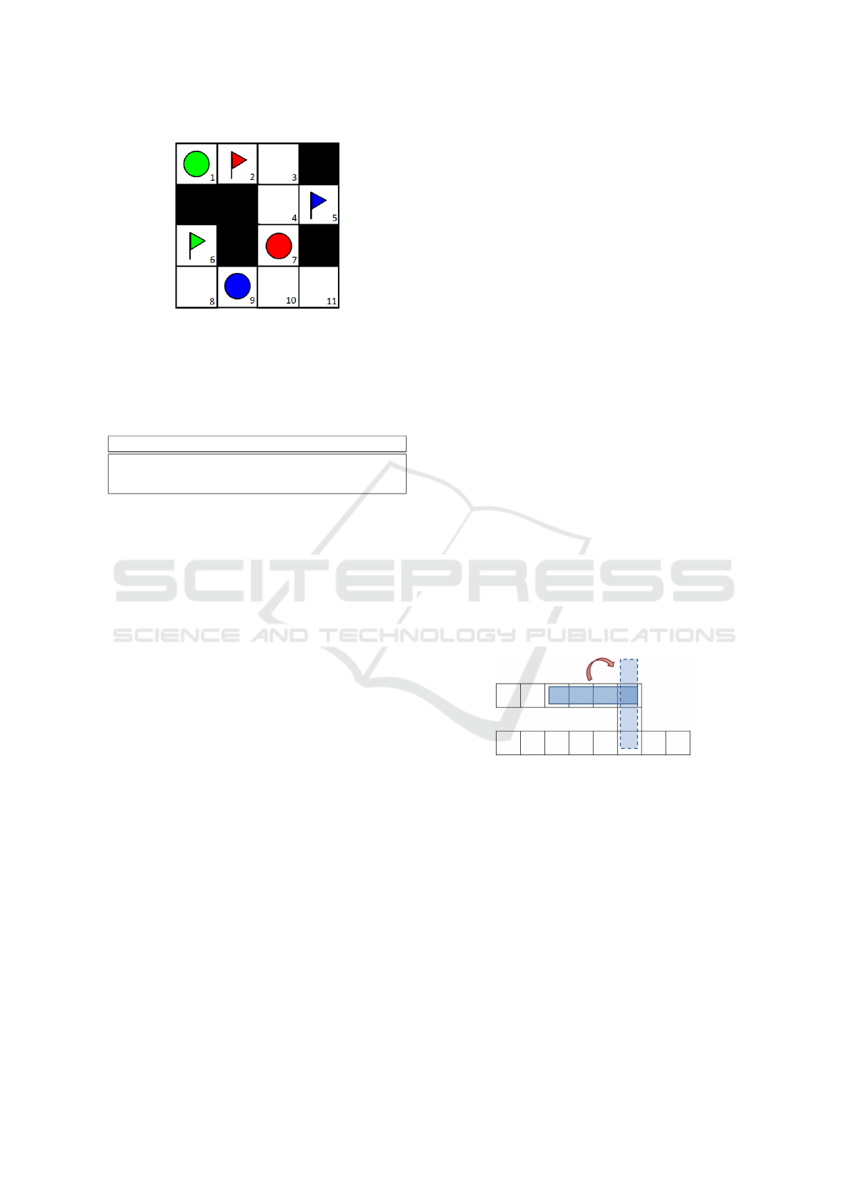
Figure 1: An example of MAPF instance. The white cells

are vertices of a 4-connected grid graph, the colored circles

denote initial locations of the agents, and the colored ﬂags

denote the goal locations of the agents.

Table 1: A solution to the MAPF instance deﬁned in Fig-

ure 1. The numbers correspond to the vertices each agent

occupies at that timestep.

Timestep 0 1 2 3 4 5 6 7 8 9

Agent Green 1 2 3 4 7 10 9 8 6 6

Agent Red 7 4 5 5 4 3 2 2 2 2

Agent Blue 9 10 11 11 11 11 10 7 4 5

2 BACKGROUND on MAPF

The multi-agent pathﬁnding (MAPF) problem is de-

ﬁned as a pair (G, A), where G is a graph G = (V, E)

and A is a set of agents. Each agent a

∈ A is deﬁned as

a pair of vertices a

= (s

, g

) which represent its start-

ing and goal vertex respectively. At each timestep, all

of the agents perform an action synchronously. The

action can be a move action to a neighboring vertex

or a wait action (i.e., staying in the same vertex).

The task is to ﬁnd a sequence of locations (alter-

natively, a sequence of actions) for each agent such

that no two agents collide with each other. There

are different types of collisions deﬁned in the liter-

ature (Stern et al., 2019). The two most often used

are vertex collision – two agents are present in the

same vertex at the same time, and swapping collision

– two agents are moving on the same edge in the op-

posite directions at the same time. Forbidding these

two collisions ensures that no two agents are present

at the exact physical location simultaneously. We call

this parallel motion since it allows the agent to move

closely one after another like a train, which will be

helpful to us. An example of a MAPF instance can be

seen in Figure 1, while a solution for that instance can

be seen in Table 1. The table states the location for

each agent at each timestep.

We do not provide a formal deﬁnition for a train

movement problem since the speciﬁc details will arise

from the formalism we use to solve the problem.

However, the task is quite intuitive and close to the

MAPF problem. We are given a shared environment

represented by a graph and a set of trains. Each train

is associated with a given initial position and the de-

sired goal position. In our models, we further assume

that each train may have a different length; therefore,

the train may occupy a different number of vertices

at a given time, each train is of length at least two,

and the trains are not allowed to move backward. The

task is to navigate each train to the desired destination

without any collision with the other trains.

2.1 Modeling Large Agents

The models proposed in this paper are built as an ex-

tension of existing MAPF models. There exist exten-

sions of the classical MAPF model to deal with large

agents, but as we shall show now, these extensions are

inappropriate to model trains of various lengths.

Generalization of MAPF for heterogeneous agents

explores the setting where each agent occupies mul-

tiple vertices in a homogeneous grid map (Atzmon

et al., 2020). With this approach, it is possible to

model a long agent that resembles a train, and while

the algorithm allows for the agent to turn, the agents

are considered to be rigid (i.e., not changing their

shape). This property may cause an instance to be

unsolvable in cases where an agent that may change

shape would be able to ﬁnd a solution. Such example

can be seen in Figure 2. The trains need to be able to

bend around corners, thus changing the shape.

Figure 2: Example of an instance that is unsolvable for a

rigid agent.

Another approach that deals with agents of vary-

ing size (Andreychuk et al., 2019), considers the

agents to be circular. In the paper, the agents move

continuously, and a collision is detected if any two

agents overlap. It is possible to model a train by a cir-

cle of sufﬁcient diameter. This representation is valid

even on bends; however, two circular agents may col-

lide in places where the physical trains are not present.

See Figure 3 for an example.

Tackling Train Routing via Multi-agent Pathﬁnding and Constraint-based Scheduling

307

Figure 3: Example of an instance that is unsolvable by rep-

resenting trains as large circular agents. The agents are

moving in opposite directions and the circular agents cause

a collision that would not happened in the physical world.

3 MODELING TRAIN

MOVEMENT

The main difference and the hardness of the problem

arise from the fact that a train may occupy more than

one location at a given time. New constraints need

to be set such that no two trains collide anywhere in

these occupied locations. Furthermore, compared to

the mentioned related work, the shape of the train may

change based on the section of the track the train is us-

ing. There exists an approach called Multi-Train Path

Finding (MTPF) (Atzmon et al., 2019) that is very

close to this problem. However, in MTPF the train ex-

pands from a start node and shrinks to the destination

node, while the trains preserve their length in reality.

We formulate two different approaches to model the

train movement.

3.1 MAPF Model

To model the trains’ movement, we treat each train

as a group of agents T

, . . . T

such that

,...T

= A.

The number of agents in each group is determined

by the length of a given train. The problem is then

to navigate the group to the goal location in such a

way that the agents not only remain connected but

also maintain the structure of the train. More specif-

ically, this means that when the group moves, each

agent moves to the location that was occupied in the

previous timestep by the agent next to it. Similarly,

if the group waits (perform no-op) each agent in the

group waits.

We start by using a MAPF solver based on a re-

duction to Boolean satisﬁability (SAT). This solver

models the classical MAPF problem as was deﬁned

in the previous chapter.

Let’s assume that we are looking for a solution to

the MAPF problem with makespan M using the par-

allel motion restriction on allowed conﬂicts. We de-

ﬁne the following two sets of variables: ∀v ∈ V, ∀a

∈

A, ∀t ∈ {0, . . . , M} : At(v, i, t) meaning that agent a

at vertex v at timestep t; and ∀(u, v) ∈ E, ∀a

∈ A, ∀t ∈

{0, . . . , M − 1} : Pass(u, v, i, t) meaning that agent a

goes through an edge (u, v) at timestep t. More specif-

ically, it starts traversing the edge at timestep t and

enters the vertex v at timestep t + 1. This is why the

variables are not deﬁned for timestep M. An auxiliary

edge (v, v) is added to E, thus Pass(v, v, i, t) means

that agent a

stays at vertex v at timestep t. To model

the MAPF problem, we introduce the following con-

straints:

∀a

∈ A : At(s

, i, 0) = 1 (1)

∀a

∈ A : At(g

, i, M) = 1 (2)

∀a

∈ A, ∀t ∈ {0, . . . , M} :

∑

v∈V

At(v, i, t) ≤ 1 (3)

∀v ∈ V, ∀t ∈ {0, . . . , M} :

∑

∈A

At(v, i, t) ≤ 1 (4)

∀u ∈ V, ∀a

∈ A, ∀t ∈ {0, . . . , M − 1} :

At(u, i, t) =⇒

∑

(u,v)∈E

Pass(u, v, i, t) = 1 (5)

∀(u, v) ∈ E, ∀a

∈ A, ∀t ∈ {0, . . . , M − 1} :

Pass(u, v, i, t) =⇒ At(v, i, t + 1) (6)

∀(u, v) ∈ E : u 6= v, ∀t ∈ {0, . . . , M − 1} :

∑

∈A

(Pass(u, v, i, t) +Pass(v, u, i, t)) ≤ 1 (7)

Constraints (1) and (2) ensure that the starting and

goal positions are valid. Constraints (3) and (4) en-

sure that each agent occupies at most one vertex and

every vertex is occupied by at most one agent. The

correct movement in the graph is forced by constraints

(5) – (7). In sequence, they ensure that if an agent is

in a certain vertex, it needs to leave it by one of the

outgoing edges (5). If an agent is using an edge, it

needs to arrive at the corresponding vertex in the next

timestep (6). Finally, (7) forbids two agents to tra-

verse two opposite edges at the same time (forbidding

swapping conﬂict). To ﬁnd the optimal makespan,

we iteratively increase M until a satisﬁable formula

is generated.

To express that the group of agents moves as a

single train, we add the following constraints.

∀j ∈ {1, . . . n}, r ∈ T

, ∀a

∈ T

, a

6= r,

∀t ∈ {0, . . . , T −1} :

∑

v∈V

Pass(v, v, r, t) =

∑

v∈V

Pass(v, v, i, t) (8)

∀j ∈ {1, . . . n}, ∀a

∈ T

, a

6= a

∀t ∈ {0, . . . , T −1}, ∀v ∈ V :

At(v, i, t) = 1 ∧ At(v, i, t + 1) = 0

=⇒ At(v, i + 1, t + 1) = 1 (9)

ICAART 2022 - 14th International Conference on Agents and Artiﬁcial Intelligence

308

Assume that there are n groups of agents (trains).

For each group, we can choose a representative r.

Also to simplify the notation, r is the ﬁrst agent in the

group, and agents’ indexes are ordered in the same

way as the agents are ordered in the train representa-

tion. This means that agent a

in a train of length l

is the agent at the very end. The constraint (8) rep-

resents a situation when the train waits. It ensures

that if one of the agents in that group is using a wait

edge, all of the agents also use wait edges. The con-

straint (9) ensures that if an agent a

moves to a new

location (i.e., it is not staying in the same location v

in two consecutive timesteps), the agent behind him,

with the index of +1, moves to the previous location v

of agent a

. The constraint that trains are not allowed

to move backward arises from constraint (9) and the

fact that trains are of length at least two – the leading

agent r of the train cannot go back as that vertex is

occupied by the second agent of the train.

Since we are considering that trains are of length

greater than one, we do not need to include the con-

straint (7) that forbids swapping of agents. Swapping

of two trains of length at least two would lead to a

vertex collision.

We provide the constraints as a set of inequalities

rather than a CNF formula since it is more readable

and there are tools that automatically translate such

inequalities into a CNF that is solvable by any SAT-

solver (Bart

ak et al., 2017).

Another idea of how one might try to simulate the

train motion is to use just one agent to represent a

train and use k-robust MAPF (Atzmon et al., 2017).

In this version of MAPF, it is required for each ver-

tex to be empty for at least k timesteps before another

agent may enter it. If k is set as the length of the

longest train, the k vertices behind each agent, where

the rest of the train should be present, are forced to

be empty, thus producing a valid plan. However, a

problem arises when the agent stops. Each timestep

the agent remains stationary the number of unusable

vertices behind the agent decreases by one. Eventu-

ally, if the agent does not move for k timesteps another

agent may move right next to it, which would create a

conﬂict in the real world. An example can be seen in

Figure 4.

3.2 Scheduling Model

Our scheduling-based model is inspired by a schedul-

ing approach for solving classical MAPF and an

extension of MAPF where edges may be assigned

lengths and capacities (Bart

ak et al., 2018).

Similarly, we model the problem in the Con-

straint Programming formalism borrowing ideas from

Figure 4: Example of 3-robust MAPF simulating train of

length 4. The agent is not performing a move action in

timesteps t, . . . , t + 3, thus the length of the simulated train

is ”shrinking”.

scheduling and routing problems. We see the possi-

ble locations as resources with limited capacity. We

use the concept of optional (alternative) activities (La-

borie et al., 2009) with specialized global constraints,

such as NoOverlap, modeling resources.

In contrast to the MAPF model, in our schedul-

ing model, we do not treat each vertex of the input

graph as a single location. This granularity is unnec-

essarily ﬁne. Considering that the railway network

usually consists of long stretches of tracks with no

intersections, we condense these long stretches into

a single location, while intersections, where the train

may change its direction to move to other rail seg-

ments, are kept with the high granularity. Figure 5

shows how a real railway network is converted to a

set of activities for a speciﬁc train. Another example

is given in the experimental section in Figure 9 show-

ing how a MAPF-like model of the railway network

is condensed in the scheduling model (vertices corre-

spond to rail segments occupied by transport activi-

ties). Note that this high abstraction is not possible in

the MAPF model, since condensing multiple vertices

into a single one would lose the information on travel

time. This is not an issue for the scheduling model,

because we can assign different durations to activities

modeling the train movement.

Figure 5: Converting a railway network to a set of transport

activities.

Given a set of n trains T

, . . . , T

and m locations

, . . . , L

created from the original graph G, we cre-

Tackling Train Routing via Multi-agent Pathﬁnding and Constraint-based Scheduling

309

ate an interval optional variable Traverse(T

, L

)

meaning that train T

is traversing location L

, coming

from location L

. It is needed to know the previous lo-

cation of the train because this can determine what are

the next possible locations and activities (recall that

trains may not simply turn around or go backward),

in other words, the previous location determines the

orientation of the train in the current location. The

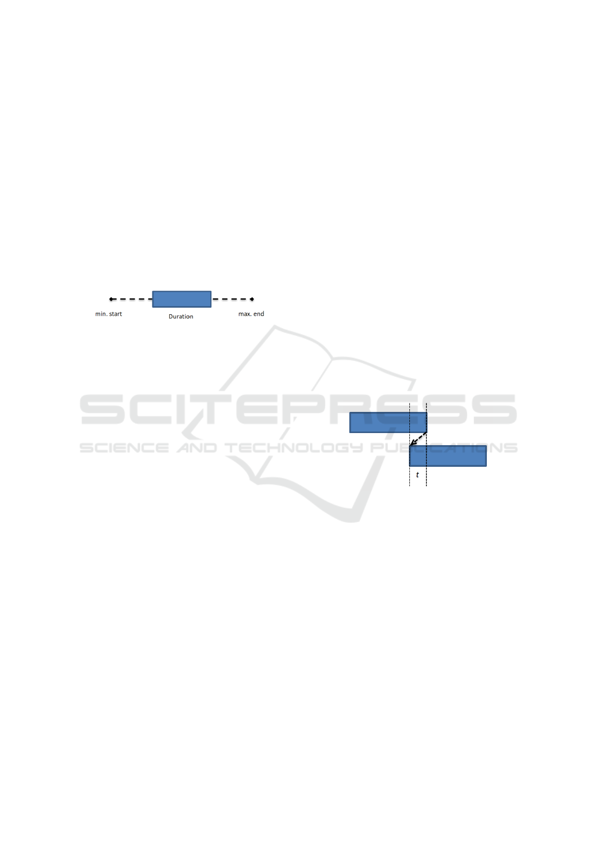
activities are interval activities, meaning that they are

assigned duration and may occur in some predeﬁned

time. See Figure 6 for visualization. The duration of

the activity is determined by the length of the train

plus the length of the rail segment and the speed of

the train. The activity directly corresponds to the time

any part of the train is present anywhere in the given

rail segment.

Figure 6: Visualization of an activity duration over the pos-

sible start and end times.

Given a start location L

of train T

, we

write Traverse(T

, L

, −) as the initial activity of

train T

. Similarly, we have the ﬁnal activity

Traverse(T

, L

) for a goal location L

of train T

In this case, the previous location is needed because

in the problem speciﬁcation we require the train to ar-

rive in the goal station with speciﬁc orientation.

The initial and ﬁnal activity of each train is re-

quired, we set the following constraints.

∀i ∈ {1, . . . , n} :

PresenceOf (Traverse(T

, L

, −)) = 1 (10)

∀i ∈ {1, . . . , n} :

PresenceOf (Traverse(T

, L

)) = 1 (11)

The presence of the other activities is determined

by the solver based on the following constraints.

∀i ∈ {1, . . . , n}, ∀j ∈ {1, . . . , m} :

Alternative(Traverse(T

, L

), Next(T

, L

))

(12)

∀i ∈ {1, . . . , n}, ∀j ∈ {1, . . . , m} :

Alternative(Traverse(T

, L

), Prev(T

, L

))

(13)

The deﬁnition of the Alternative constraint, which

gets an interval variable as the ﬁrst argument and a

set of interval variables as the second argument, is as

follows. If the activity given as the ﬁrst argument is

present, then exactly one activity from the set of ac-

tivities given as the second argument is present. In

addition, it gives a constraint on the start and end time

of the activities. The constraints (12) and (13) ensure

that if an agent is traversing a location, it will next tra-

verse one of the possible adjacent locations given the

orientation of the train. Similarly, before traversing a

location, the train needed to be traversing one of the

locations that can lead it to the current one. The Pos-

sible transitions between activities need to be ﬁgured

out as an input of the model. However, this is easily

done by a simple traversal of the underlying graph.

The start and end times of the following activities

need to be set. To ensure the correct movement of the

trains with no swapping of the trains, we introduce

a negative time delay between the two following ac-

tivities. See Figure 7 for an illustration. In the ﬁrst

activity the train is traversing one rail segment, while

in the other activity, the train is traversing some adja-

cent rail segment. During the t timesteps the train is

performing both activities; the train is in fact occupy-

ing both rail segments at the same time. Therefore this

time delay is determined by the length of the train and

train speed. Basically, it deﬁnes the time that the train

needs to pass a border point between two successive

railway segments.

Figure 7: Visualization of two activities being performed

after each other with the negative time delay t.

The negative time delay is enough to enforce no

swapping among the trains. To forbid the trains to oc-

cupy the same location at the same time, we use the

NoOverlap constraint on the activities that occur at

the same location. This constraint ensures that trans-

port activities of different trains for the same rail seg-

ment (location) do not overlap in time – the trains are

not using that segment at the same time.

∀j ∈ {1, . . . , m} :

NoOverlap(

[

,...,T

Traverse(T

, L

) (14)

3.3 Comparison of the Models

The two proposed models both abstract the train

movement; however, there are slight differences be-

tween what is possible to model by each model. The

ICAART 2022 - 14th International Conference on Agents and Artiﬁcial Intelligence

310

MAPF model can express the position of the whole

train at each timestep very precisely. In contrast, the

scheduling model only provides which location (rail

segment) of the network is traversed at each time, but

the train’s exact location at that rail segment is not

given. This degree of imprecision can be changed

based on the granularity of the locations created.

The MAPF model allows the trains to visit any

vertex in the grid any number of times. On the other

hand, the scheduling model allows using each activity

only once. This property means that the train cannot

return to a given location with the same orientation.

This issue can be solved by creating extra activities

with a unique name for the given location to allow the

train to return. A change to the following possible

locations is then needed. However, it is usually not

necessary in a real-world setting for a train to move in

a loop to reach its destination.

While the last two properties were shortcomings

of the scheduling model (the model does not support

planning entirely), this model can represent broader

scenarios than the classical MAPF model. For exam-

ple, by setting the transfer times and duration of each

activity, we can simulate different speeds for each

train. Furthermore, we can impose different travel

speeds for each location. Similarly, we can also sim-

ulate speeding up and slowing down the train in the

locations leading to the stations. Also, required vis-

ited locations may be set by using the PresenceOf

constraint. The exact time of visit is then left to the

solver. On the other hand, if we know in advance the

time window when this required visit needs to occur

(for example, from the given timetable), we can also

set it by changing the minimal start and maximal end

times of the activity.

4 EXPERIMENTAL EVALUATION

To test the proposed modeling methods, we imple-

mented the scheduling approach in the IBM CP Op-

timizer version 12.8 (Laborie, 2009). For the SAT-

based approach we used the Picat language and com-

piler version 2.7b7 (Bart

ak et al., 2017). The experi-

ments were run on a PC with an AMD Ryzen 7 4700U

running at 2.00 GHz with 16 GB of RAM. We used a

cutoff time of 300 seconds per problem instance.

4.1 Instances

Classical MAPF techniques are frequently compared

using grid-based benchmark maps (Stern et al., 2019).

However, these maps are far from maps represent-

ing train networks. Flatland challenge maps (Mo-

hanty et al., 2020) describe railway networks, but they

are designed for unit-size agents and do not repre-

sent well stations with multiple platforms. Therefore,

we created three 4-connected grid maps representing

a structure of a rail network inspired by the Flatland

challenge maps, but with more detailed train stations

(see Figure 8). Each of the maps consists of three sta-

tions (represented by the red highlight), each with ﬁve

rail tracks of length ﬁve units. The stations represent

a location where a train may start and end after the

execution of the found plan. In total there are ﬁfteen

possible starting and goal locations on each map. We

created the maximal number of agents (ﬁfteen) of ran-

dom length between two and ﬁve for each map. The

start location was placed at random and the goal loca-

tion was also chosen by random from one of the other

two stations. Note that the orientation of the train is

also an important part of the start and goal location.

This process was done ﬁve times with different ran-

dom seeds. Each instance is then created by consid-

ering a different number of trains, from one to ﬁfteen,

on the given map. In total, this produces 225 different

instances.

The representation for the MAPF model is quite

straightforward. Each vertex in the map represents a

location. Each train with length l consists of l agents

with assigned start and goal locations such that the

orientation of the train is maintained.

For the scheduling model, we ﬁrst needed to split

the grid map into locations. If each vertex was a sin-

gle location, we would lose the strength of the model,

so instead, we considered a sequence of vertices with

only two neighbors as a single location. Example of

such transformation of map Linear can be seen in Fig-

ure 9. Note that this transformation is only needed due

to comparison with the MAPF-like approach. In real-

ity, the railway network is given as a graph of tracks

(Figure 5).

Over each of the locations, an activity was created

for each train. The minimal start and maximal end of

the activity were set to 0 and an upper bound on the

whole plan. The duration of the activity was set as the

length of the train plus the length of the location (i.e.,

the number of vertices in that location). The transfer

time was set as the length of the train. Using clever

preprocessing, the bounds on the start and end times

of the activity may be improved, however, in our ex-

periments, we did not ﬁnd this to be the bottleneck for

the solver.

Since the two models do not provide exactly the

same solutions, as we discussed at the end of the last

section, and we do not look for an optimal solution,

we do not increase the upper bound on makespan T

in the SAT model by 1. Rather, we increase the T

Tackling Train Routing via Multi-agent Pathﬁnding and Constraint-based Scheduling

311

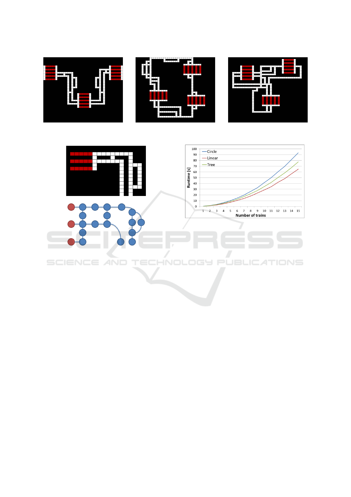
(a) Linear. (b) Circle. (c) Tree.

Figure 8: Maps used in the experiments.

Figure 9: In the top is part of the Linear map. On the bottom

is its representation as locations that the scheduling model

uses. Note that the long sequences of vertices with just two

neighbours are abstracted as a single location.

by the length of the longest train, which is ﬁve in our

instances. The reasoning behind this is that if there

is no solution in a given lower bound on makespan, it

may be caused either by a conﬂict of two trains or by

the fact that a train is required to arrive at the station

from a different direction. Waiting for a train to free

a given vertex takes the same number of timesteps as

is the length of the train. Arriving at a station from a

different direction means going around the station. In

both cases increasing the T by just 1 would not help.

Of course, this approach does not guarantee ﬁnding

a makespan-optimal solution, but it should be able to

ﬁnd a solution in less computational time.

4.2 Results

Out of the 225 instances, the SAT MAPF model was

able to solve only 38 with the most trains solved be-

ing 5 on map Tree. On the other hand, the scheduling

model was able to solve all of the instances using just

a fraction of the allowed runtime. Figure 10 shows the

Figure 10: Measured runtime for the scheduling approach.

The presented values are average runtime of instances with

a given number of agents.

average runtime per number of trains. The results are

split for the three different types of maps. From these

results, we can see that the runtime increases with the

number of trains being present in the graph, as is ex-

pected. We also observe that the different structure of

the maps gives a clear ordering in hardness of the in-

stances with Linear being the easiest, while Circle is

the hardest. We can observe the same ordering in the

SAT model results.

Such poor performance by the SAT-based model

was not expected. We performed the experiments

again without the constraint on agents modeling a

train to remain connected. Thus a classical MAPF

problem was being solved. This relaxation was able

to solve 111 instances out of 225. This is a substan-

tial improvement, however, it is still far away from

solving all of the instances as the scheduling model is

able to. From this result, we can draw the conclusion

that the added constraints on the train movement are

hard for the solver. Furthermore, we can see that this

type of instance is hard even for classical MAPF. In-

deed, when 13 trains are present (which was the maxi-

mal number solved in this experiment by the classical

MAPF algorithm), there are up to 65 single agents on

the map. The map itself provides a challenging envi-

ronment where the agents do not have much space to

avoid each other.

ICAART 2022 - 14th International Conference on Agents and Artiﬁcial Intelligence

312

5 CONCLUSION

In this paper, we studied the problem of train routing

in a shared environment. We proposed two models.

The ﬁrst one is based on a classical MAPF reduction-

based approach. In this approach, each train is mod-

eled as a group of agents moving to the goal loca-

tion in a connected manner, simulating the position

of the whole train. Our second model is inspired by a

scheduling problem, where the graph is split into con-

tinuous locations – rail segments. Each activity rep-

resents a traversal of a given location by a train. The

activities are intertwined in such a manner to ensure

that the trains do not perform a forbidden movement;

speciﬁcally, they do not occupy the exact physical lo-

cation at the same time.

We compared the two models by their ability to

model the real world. It seems that the scheduling

model can represent a wider variety of real-world at-

tributes, such as different speeds in any segment of

the rail network. On the other hand, it is more com-

plicated to create the instance for this model automat-

ically from the grid-like MAPF maps

We also evaluated the models empirically and

found that the MAPF model does not scale well over

instances with just a few trains. On the other hand, the

scheduling model solved all of the instances in just a

fraction of the allocated runtime, showing great po-

tential.

ACKNOWLEDGEMENTS

This research is supported by the Czech-USA Coop-

erative Scientiﬁc Research Project LTAUSA19072.

REFERENCES

Andreychuk, A., Yakovlev, K. S., Atzmon, D., and Stern, R.

(2019). Multi-agent pathﬁnding with continuous time.

In Kraus, S., editor, 28th International Joint Confer-

ence on Artiﬁcial Intelligence (IJCAI), pages 39–45.

ijcai.org.

Atzmon, D., Diei, A., and Rave, D. (2019). Multi-train

path ﬁnding. In Surynek, P. and Yeoh, W., edi-

tors, 12th International Symposium on Combinatorial

Search (SOCS), pages 125–129. AAAI Press.

Atzmon, D., Felner, A., Stern, R., Wagner, G., Bart

ak,

R., and Zhou, N. (2017). k-robust multi-agent path

ﬁnding. In Fukunaga, A. and Kishimoto, A., edi-

tors, 10th International Symposium on Combinatorial

Search (SOCS), pages 157–158. AAAI Press.

Atzmon, D., Zax, Y., Kivity, E., Avitan, L., Morag, J.,

and Felner, A. (2020). Generalizing multi-agent path

ﬁnding for heterogeneous agents. In Harabor, D. and

Vallati, M., editors, 13th International Symposium on

Combinatorial Search (SOCS), pages 101–105. AAAI

Press.

Bart

ak, R., Svancara, J., and Vlk, M. (2018). A scheduling-

based approach to multi-agent path ﬁnding with

weighted and capacitated arcs. In Andr

e, E., Koenig,

S., Dastani, M., and Sukthankar, G., editors, 17th In-

ternational Conference on Autonomous Agents and

MultiAgent Systems (AAMAS), pages 748–756.

Bart

ak, R., Zhou, N.-F., Stern, R., Boyarski, E., and

Surynek, P. (2017). Modeling and solving the multi-

agent pathﬁnding problem in picat. In 29th IEEE In-

ternational Conference on Tools with Artiﬁcial Intel-

ligence (ICTAI), pages 959–966. IEEE Computer So-

ciety.

Laborie, P. (2009). IBM ILOG CP optimizer for detailed

scheduling illustrated on three problems. In van Ho-

eve, W. J. and Hooker, J. N., editors, 6th Interna-

tional Conference on Integration of AI and OR Tech-

niques in Constraint Programming for Combinatorial

Optimization Problems (CPAIOR), volume 5547 of

Lecture Notes in Computer Science, pages 148–162.

Springer.

Laborie, P., Rogerie, J., Shaw, P., and Vil

ım, P. (2009). Rea-

soning with conditional time-intervals. part ii: An al-

gebraical model for resources. In 22nd Florida AI Re-

search Society Conference (FLAIRS), pages 201–206.

Li, J., Chen, Z., Zheng, Y., Chan, S., Harabor, D., Stuckey,

P. J., Ma, H., and Koenig, S. (2021). Scalable rail plan-

ning and replanning: Winning the 2020 ﬂatland chal-

lenge. In Biundo, S., Do, M., Goldman, R., Katz, M.,

Yang, Q., and Zhuo, H. H., editors, 31st International

Conference on Automated Planning and Scheduling

(ICAPS), pages 477–485. AAAI Press.

Mohanty, S. P., Nygren, E., Laurent, F., Schneider, M.,

Scheller, C., Bhattacharya, N., Watson, J. D., Egli,

A., Eichenberger, C., Baumberger, C., Vienken, G.,

Sturm, I., Sartoretti, G., and Spigler, G. (2020).

Flatland-rl : Multi-agent reinforcement learning on

trains. CoRR, abs/2012.05893.

Stern, R., Sturtevant, N. R., Felner, A., Koenig, S., Ma, H.,

Walker, T. T., Li, J., Atzmon, D., Cohen, L., Kumar,

T. K. S., Bart

ak, R., and Boyarski, E. (2019). Multi-

agent pathﬁnding: Deﬁnitions, variants, and bench-

marks. In Surynek, P. and Yeoh, W., editors, 12th

International Symposium on Combinatorial Search

(SOCS), pages 151–159. AAAI Press.

Tackling Train Routing via Multi-agent Pathﬁnding and Constraint-based Scheduling

313