The MVTec 3D-AD Dataset for Unsupervised 3D Anomaly Detection and

Localization

Paul Bergmann

1,2 a

, Xin Jin

3 b

, David Sattlegger

1 c

and Carsten Steger

1 d

MVTec Software GmbH, Germany

Technical University of Munich, Germany

Karlsruhe Institute of Technology, Germany

Keywords:

Anomaly Detection, Dataset, Unsupervised Learning, Visual Inspection, 3D Computer Vision.

Abstract:

We introduce the ﬁrst comprehensive 3D dataset for the task of unsupervised anomaly detection and localization.

It is inspired by real-world visual inspection scenarios in which a model has to detect various types of defects

on manufactured products, even if it is trained only on anomaly-free data. There are defects that manifest

themselves as anomalies in the geometric structure of an object. These cause signiﬁcant deviations in a 3D

representation of the data. We employed a high-resolution industrial 3D sensor to acquire depth scans of 10

different object categories. For all object categories, we present a training and validation set, each of which

solely consists of scans of anomaly-free samples. The corresponding test sets contain samples showing various

defects such as scratches, dents, holes, contaminations, or deformations. Precise ground-truth annotations are

provided for every anomalous test sample. An initial benchmark of 3D anomaly detection methods on our

dataset indicates a considerable room for improvement.

1 INTRODUCTION

The increased availability and precision of modern 3D

sensors has led to signiﬁcant advances in the ﬁeld of

3D computer vision. The research community has used

these devices to create datasets for a wide variety of

real-world problems, such as point cloud registration

(Zeng et al., 2017), classiﬁcation (Wu et al., 2015), 3D

semantic segmentation (Chang et al., 2015; Dai et al.,

2017), 3D object detection (Armeni et al., 2016), and

rigid pose estimation (Drost et al., 2017; Hoda

n et al.,

2020). The development of new and improved algo-

rithms relies on the availability of such high quality

datasets.

A task of particular importance in many applica-

tions is to recognize anomalous data that deviates from

what a model has previously observed during training.

In manufacturing, for example, these kinds of methods

can be used to detect defects during inference, while

only being trained on anomaly-free samples. In au-

tonomous driving, it is safety critical that an intelligent

https://orcid.org/0000-0002-4458-3573

https://orcid.org/0000-0002-2078-8056

https://orcid.org/0000-0002-8336-4672

https://orcid.org/0000-0003-3426-1703

system can detect structures it has not seen during

training. This problem has attracted signiﬁcant atten-

tion for color or grayscale images. Curiously, the ﬁeld

of unsupervised anomaly detection is comparatively

unexplored in the 3D domain. We believe that a key

reason for this is the unavailability of suitable datasets.

To ﬁll this gap and spark further interest in the de-

velopment of new methods, we introduce a real-world

dataset for the task of unsupervised 3D anomaly de-

tection and localization. Given a set of exclusively

anomaly-free 3D scans of an object, the task is to

detect and localize various types of anomalies. Our

dataset is inspired by industrial inspection scenarios.

This application has been identiﬁed as an important

use case for the task of unsupervised anomaly detec-

tion because the nature of all possible defects that may

occur in practice is often unknown. In addition, defec-

tive samples for training can be difﬁcult to acquire and

precise labeling of defects is a laborious task. Figure 1

shows two prototypical samples of our new dataset.

Our main contributions are as follows:

•

We introduce the ﬁrst comprehensive dataset for

unsupervised anomaly detection and localization

in three-dimensional data. It consists of 4147 high-

resolution 3D point cloud scans from 10 real-world

202

Bergmann, P., Jin, X., Sattlegger, D. and Steger, C.

The MVTec 3D-AD Dataset for Unsupervised 3D Anomaly Detection and Localization.

DOI: 10.5220/0010865000003124

In Proceedings of the 17th International Joint Conference on Computer Vision, Imaging and Computer Graphics Theory and Applications (VISIGRAPP 2022) - Volume 5: VISAPP, pages

202-213

ISBN: 978-989-758-555-5; ISSN: 2184-4321

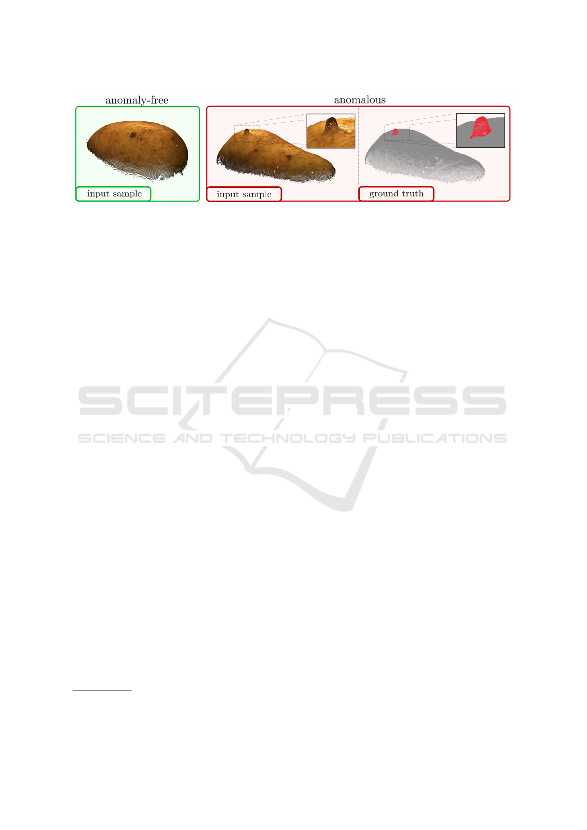
Figure 1: Two samples representing the category potato of our new dataset. The sample on the left is anomaly-free while the

one on the right contains a nail stuck through the surface of the potato. We depict the point clouds overlaid with the associated

color values. For the anomalous sample, we additionally display the annotated ground truth.

object categories. While the training and validation

sets only contain anomaly-free data, the samples

in the test set contain various types of anomalies.

Precise ground truth annotations are provided for

each anomaly.

•

We evaluate current methods that were speciﬁcally

designed for unsupervised 3D anomaly localiza-

tion. Our initial benchmark reveals that existing

methods do not perform well on our dataset and

that there is considerable room for future improve-

ment.

2 RELATED WORK

Anomaly Detection in 2D.

For two-dimensional im-

age data, numerous synthetic and real-world bench-

mark datasets exist. They cover various domains,

e.g., autonomous driving (Blum et al., 2019), video

anomaly detection (Li et al., 2013; Lu et al., 2013;

Sultani et al., 2018), or industrial inspection scenarios.

Since we propose a new industrial inspection

dataset, we focus our summary on existing datasets

from this domain. The task is to detect and localize

defects on manufactured products when only a set of

anomaly-free training images is available. Huang et al.

(2018) present a surface inspection dataset of 1344

images of magnetic tiles. Test images contain various

types of anomalies, such as cracks or uneven areas.

Similar datasets exist that focus on the inspection of

a single repetitive two-dimensional texture (Carrera

et al., 2017; Song and Yan, 2013; Wieler and Hahn,

2007). Bergmann et al. (2019a, 2021) introduce a more

comprehensive dataset that contains a total of 5354 im-

ages showing instances of ﬁve texture and ten object

categories. The test set contains 73 distinct types of

anomalies, such as contaminations or scratches on the

manufactured products.

The dataset will be made publicly available at

https://www.mvtec.com/company/research/datasets.

The aforementioned datasets have led to the de-

velopment of numerous methods that are intended to

operate on 2D color images. A popular approach

(Bergmann et al., 2020; Cohen and Hoshen, 2021;

Salehi et al., 2021; Wang et al., 2021) is to model the

distribution of descriptors extracted from neural net-

works pretrained on large-scale datasets like ImageNet

(Krizhevsky et al., 2012). Networks that are pretrained

in such a way expect RGB images as input. The re-

sulting methods are therefore ill-suited to process 2D

representations of 3D data, such as depth images, and

cannot be easily transferred to 3D anomaly detection.

A different line of work uses generative models such as

convolutional autoencoders (AEs) (Masci et al., 2011)

or generative adversarial networks (GANs) (Goodfel-

low et al., 2014) to detect anomalies by evaluating a

pixelwise reconstruction error. Schlegl et al. (2019)

introduce f-AnoGAN, where a GAN is trained on the

anomaly-free training data. In a second step, an en-

coder network is trained to output latent samples that

reconstruct the respective input images when passed

to the generator of the GAN. Similarly, methods based

on autoencoders (Bergmann et al., 2019b; Park et al.,

2020) ﬁrst encode input images with a low dimensional

latent sample, and then decode that sample to minimize

a pixelwise reconstruction error. For both approaches,

anomaly scores are computed by a pixelwise compar-

ison of an input image with its reconstruction. Since

these methods do not require a domain-speciﬁc pre-

training, they can be adapted to other two-dimensional

representations, such as depth images.

Anomaly Detection in 3D.

To date, there exists no

comprehensive 3D dataset designed explicitly for the

unsupervised detection and localization of anomalies.

Existing methods for this problem are evaluated on

two medical benchmarks that were originally intro-

duced for the supervised detection of diseases in brain

magnetic resonance (MR) scans. Menze et al. (2015),

Bakas et al. (2017), and Baid et al. (2021) present the

multimodal brain tumor image segmentation bench-

The MVTec 3D-AD Dataset for Unsupervised 3D Anomaly Detection and Localization

203

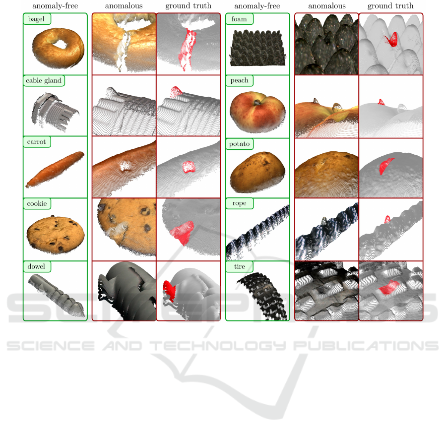
Figure 2: Examples for all 10 dataset categories of the MVTec 3D-AD dataset. For each category, the left column shows an

anomaly-free point cloud with RGB values projected onto it. The second column shows a close-up view of an anomalous test

sample. Anomalous points are highlighted in the third column in red. Note that the background planes were removed for better

visibility.

mark (BRATS). It consists of 65 multi-contrast MR

scans from glioma patients. Each sample is provided

as a dense voxel grid and tumors were annotated by

radiologists in each image slice of the scan. Similarly,

Liew et al. (2018) provide the Anatomical Tracings of

Lesions After Stroke (ATLAS) dataset. It consists of

304 MR scans with corresponding ground truth anno-

tations of brain lesions. Both these datasets provide

3D information by stacking multiple grayscale images

to form a dense voxel grid. Hence, the nature of this

data is fundamentally different from the one in our

dataset that describes the geometric surface of objects.

Due to the lack of more diverse 3D datasets for

unsupervised anomaly detection, there exist only very

few methods designed for this task. Only recently,

Simarro Viana et al. (2021) introduced an extension

of f-AnoGAN to voxel data. As for the 2D case, a

GAN is trained to generate voxel grids that mimic the

training distribution using 3D convolutions. Subse-

quently, an encoder network is trained that maps input

samples to the corresponding latent samples of the gen-

erator. During inference, anomaly scores are derived

for each voxel element by comparing the input voxel

to the reconstructed one. Bengs et al. (2021) present

an autoencoder-based method that also operates on

voxel grids. A variational autoencoder is trained to

reconstruct voxel grids through a low-dimensional la-

tent variable. Anomaly scores are again derived by a

per-voxel comparison of the input to its reconstruction.

3 DESCRIPTION OF THE

DATASET

The MVTec 3D-AD dataset consists of 4147 scans

acquired by a high-resolution industrial 3D sensor. For

each of the 10 object categories, a set of anomaly-free

scans is provided for model training and validation.

The test set contains both, anomaly-free scans as well

as object samples that contain various types of anoma-

lies, such as scratches, dents, or contaminations. The

defects were devised and fabricated as they would

VISAPP 2022 - 17th International Conference on Computer Vision Theory and Applications

204

Table 1: Statistical overview of the MVTec 3D-AD dataset. For each category, we list the number of training, validation,

and test images. Test images are split into anomaly-free images and images containing anomalies. We report the number of

different defect types, the number of annotated regions, and the size of the (x, y, z) images for each category.

Category # Train

# Val

# Test

(good)

# Test

(anomalous)

# Defect

types

# Annotated

regions

Image size

(width × height)

bagel 244 22 22 88 4 112 800 × 800

cable gland 223 23 21 87 4 90 400 × 400

carrot 286 29 27 132 5 159 800 × 800

cookie 210 22 28 103 4 128 500 × 500

dowel 288 34 26 104 4 131 400 × 400

foam 236 27 20 80 4 115 900 × 900

peach 361 42 26 106 5 131 600 × 600

potato 300 33 22 92 4 115 800 × 800

rope 298 33 32 69 3 72 900 × 400

tire 210 29 25 87 4 95 600 × 800

total 2656 294 249 948 41 1148

occur in real-world inspection scenarios.

Five of the object categories in our dataset exhibit

considerable natural variations from sample to sam-

ple. These are bagel, carrot, cookie, peach, and potato.

Three more objects, foam, rope, and tire, have a stan-

dardized appearance but can be easily deformed. The

two remaining objects, cable gland and dowel, are

rigid. In principle, inspecting the last two could be

achieved by comparing an object’s geometry to a CAD

model. However, unsupervised methods should be

able to detect anomalies on all kinds of objects and

the creation of a CAD model might not always be

desirable or practical in a real application. An exam-

ple point cloud for each dataset category is shown in

Figure 2. The ﬁgure also displays some anomalies

together with the corresponding ground truth annota-

tions. The images of the bagel and the cookie show

cracks in the objects. The surfaces of the cable gland

and the dowel exhibit geometrical deformations. There

is a hole in the carrot and some contaminations on the

peach and the rope. Parts of the foam, the potato, and

the tire are cut off. These are prototypical examples of

the 41 types of anomalies present in our dataset. More

statistics on the dataset are listed in Table 1.

3.1 Data Acquisition and Preprocessing

All dataset scans were acquired with a Zivid One

Medium,

an industrial sensor that records high-

resolution 3D scans using structured light. The data

is provided by the sensor as a three-channel image

with a resolution of 1920

1200 pixels. The channels

represent the

, and

coordinates with respect to

the local camera coordinate frame. The

(x, y, z)

val-

ues of the image provide a one-to-one mapping to the

https://www.zivid.com/zivid-one-plus-medium-3d-

camera

corresponding point cloud. In addition, the sensor ac-

quires complementary RGB values for each

(x, y, z)

pixel. It was statically mounted to view all objects

of each individual category from the same angle. We

performed a calibration of the internal camera parame-

ters that allows to project 3D points into the respective

pixel coordinates (Steger et al., 2018). The scene was

illuminated by an indirect and diffuse light source.

For each dataset category, we speciﬁed a ﬁxed rect-

angular domain and cropped the original

(x, y, z)

and

RGB images to reduce the amount of background pix-

els in the samples. The acquisition setup as well as the

preprocessing are very similar to real-world applica-

tions where an object is usually located in a deﬁned

position and the illumination is chosen to best suit the

task. In addition, our setup enables and simpliﬁes data

augmentation. All objects were recorded on a dark

background and the preprocessing leaves a sufﬁcient

margin around the objects to allow for the applica-

tion of various data augmentation techniques, such

as crops, translations, or rotations. This enables the

use of our dataset for the training of data-hungry deep

learning methods, as demonstrated by our experiments

in Section 4.

Figure 3 shows the data provided for the anoma-

lous test sample of the peach displayed in Figure 2.

The image is of size 600

600 pixels, cropped from the

original sensor scan. The ﬁrst three images visualize

the

, and

coordinates of the dataset sample, respec-

tively. White pixels mark areas where the sensor did

not return any 3D information due to, e.g., occlusions,

reﬂections, or sensor inaccuracies. The correspond-

ing RGB and ground truth annotation images are also

displayed.

The MVTec 3D-AD Dataset for Unsupervised 3D Anomaly Detection and Localization

205

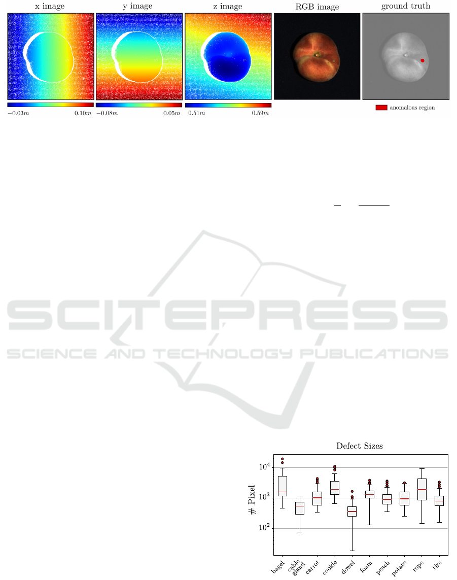
Figure 3: Visualization of the provided data for one anomalous test sample of the dataset category peach. In addition to three

images that encode the 3D coordinates of the object, RGB information as well as a pixel-precise ground-truth image are

provided.

3.2 Ground-truth Annotations

We provide precise ground-truth annotations for each

anomalous sample in the test set. Anomalies were

annotated in the 3D point clouds. Since there is a one-

to-one mapping of the 3D points to their respective

pixel locations in the

(x, y, z)

image, we make the an-

notations available as two-dimensional regions. This

procedure allows us to additionally label invalid sensor

pixels and thus annotate anomalies that manifest them-

selves through the absence of points. For example,

an anomaly might lead to a failure of 3D reconstruc-

tion and therefore yield invalid pixels in the 3D image.

Furthermore, if an anomaly is visible in the RGB im-

age and its corresponding color pixels are not already

included in the ground truth label, we append these

pixels to the annotation.

An example ground truth mask is shown in Fig-

ure 3, where a contamination is present on the peach.

In Figure 2, further annotations are visualized when

projected to the valid 3D points of a scene. The size

of the individual connected components of the anoma-

lies present in the test set varies greatly, from a few

hundred to several thousand pixels. Figure 4 visual-

izes their distribution as a box-and-whisker plot with

outliers on a logarithmic scale (Tukey, 1977).

3.3 Performance Evaluation

To assess the anomaly localization performance of a

method on our dataset, we require it to output a real-

valued anomaly score for each

(x, y, z)

pixel of the test

set. In contrast to only assigning anomaly scores to all

valid 3D points of the test samples, this allows the de-

tection of anomalies that manifest themselves through

invalid sensor pixels or missing 3D structures. These

anomaly scores are converted to binary predictions

using a threshold. We then compute the per-region

overlap (PRO) metric (Bergmann et al., 2021), which

is deﬁned as the average relative overlap of the binary

prediction

with each connected component

of the

ground truth. The PRO value is computed as

PRO =

∑

k=1

|P ∩C

, (1)

where

is the total number of ground truth compo-

nents. This process is repeated for multiple thresholds

and a curve is constructed by plotting the resulting

PRO values against the corresponding false positive

rates. The ﬁnal performance measure is computed by

integrating this curve up to a limited false positive rate

and normalizing the resulting area to the interval

[0, 1]

This is a standard metric for the task of unsupervised

anomaly localization and is particularly useful when

anomalies vary signiﬁcantly in size.

We want to stress that, when working with our

dataset, we strongly discourage to calculate the area

under the PRO curve up to high false positive rates.

We recommend to select the integration limit no larger

than 0.3. This is due to the fact that the anomalous

regions are very small compared to the size of the

images. At large false positive rates, the amount of

erroneously segmented pixels would be signiﬁcantly

Figure 4: Size of anomalies for all objects in the dataset visu-

alized as a box-and-whisker plot. Defect areas are reported

as the total number of pixels within an annotated connected

component. Anomalies vary greatly in size for each dataset

category.

VISAPP 2022 - 17th International Conference on Computer Vision Theory and Applications

206

larger than the number of actually anomalous pixels.

This would lead to segmentation results that are no

longer meaningful in practice.

Our dataset can also be used to assess the perfor-

mance of algorithms that make a binary decision for

each sample if it contains an anomaly or not. In this

case, we report the area under the ROC curve as a

standard classiﬁcation metric.

4 INITIAL BENCHMARK

To examine how existing 3D anomaly localization

methods perform on our new dataset, we conducted an

initial benchmark. It is intended to serve as a baseline

for future methods. Very few methods have been pro-

posed explicitly for this task and all of them operate

on voxel data. This is mainly due to the fact that these

methods are originally intended to process MR or CT

scans that consist of several layers of intensity images.

As representatives from this class of methods, we in-

clude Voxel f-AnoGAN (Simarro Viana et al., 2021)

and our own implementation of a convolutional Voxel

AE (Bengs et al., 2021) in our benchmark. Predeces-

sors of these methods were developed for 2D image

data. The main difference between the 2D and 3D

methods is the use of 2D convolutions on images and

3D convolutions on voxel data, respectively. There-

fore, these methods are easily adapted to process depth

images and we include them in our benchmark as well.

In addition to these deep learning methods, we evalu-

ate the performance of variation models (Steger et al.,

2018) on voxel data and depth images. They detect

anomalies by calculating the pixel- or voxel-wise Ma-

halanobis distance to the training data distribution.

All evaluated methods can either operate solely on

the 3D data or can additionally process the color infor-

mation attached to each 3D point. We therefore also

compare the difference in performance when adding

color information to the models. Detailed information

on training parameters and model architectures can be

found in the Appendix.

4.1 Training and Evaluation Setup

Data Representation.

To represent dataset samples

as voxel grids, we ﬁrst compute a global 3D bound-

ing box over the entire training set for each dataset

category. Then, a grid of

n × n × n

voxels is placed

at the center of the bounding box. The side length of

the grid is is chosen to be equal to the longest side

Evaluation scripts for the computation of all above

performance measures will be published together with the

dataset.

of the bounding box. If only 3D data is processed,

occupied and empty voxels are assigned the values

and

−1

, respectively. If RGB information is added,

empty voxels are assigned the vector

(−1, −1, −1)

Occupied voxels are assigned the average RGB value

of all points that fall inside the same grid cell.

For methods that process depth images, we com-

pute the euclidean distance to the camera center for

each valid pixel in the original

(x, y, z)

images. Invalid

pixels are assigned a distance of

. If color informa-

tion is included, the RGB channels are appended to

the single-channel depth image. For both, the voxel

grids and depth images, the RGB values are scaled to

the interval [0, 1].

Methods on Voxel Grids.

For all voxel-based meth-

ods, we use grids of size

64 × 64 × 64

voxels, as pro-

posed by Simarro Viana et al. (2021). To choose the

latent dimension of the compression-based methods,

we performed an ablation study, which is included in

the Appendix. Anomaly scores are computed by a

voxel-wise comparison of the input with its reconstruc-

tion.

The voxel grids of the samples of our dataset are

sparsely populated and the majority of voxels is empty.

We found that this leads to problems when training

the Voxel AE if each voxel is weighted equally in the

reconstruction loss. In this case, the model tends to

simply output an empty voxel grid to minimize the

reconstruction error. To address this imbalance, we

introduce a loss weight

w ∈ (0, 1)

that is computed as

the fraction of empty voxels in the training set. During

training, the loss at each voxel is then multiplied by

if the voxel is occupied and by (1 − w) otherwise.

For the Voxel Variation Model, we ﬁrst compute

the mean and standard deviation of the training data

at each voxel. During inference, anomaly scores are

derived by computing the voxel-wise Mahalanobis

distance of each test sample to the training distribution.

Methods on Depth Images.

Our implementations

of Depth f-AnoGAN and the Depth AE both process

images at a resolution of

256 × 256

pixels. Input im-

ages are zoomed using nearest neighbor interpolation

for depth, and bilinear interpolation for color images.

Anomaly scores are derived by a per-pixel compari-

son of the input images and their reconstructions. The

Depth Variation Model processes images with their

original resolution and computes the mean and stan-

dard deviation over the entire training set at each image

pixel. Again, anomaly scores are derived by com-

puting the pixel-wise Mahalanobis distance from the

training distribution.

The MVTec 3D-AD Dataset for Unsupervised 3D Anomaly Detection and Localization

207

Table 2: Anomaly localization results. The area under the PRO curve is reported for an integration limit of

0.3

for each

evaluated method and dataset category. The best performing methods are highlighted in boldface.

bagel

cable

gland

carrot cookie dowel foam peach potato rope tire mean

3D Only

Voxel

GAN 0.440 0.453 0.825 0.755 0.782 0.378 0.392 0.639 0.775 0.389 0.583

AE 0.260 0.341 0.581 0.351 0.502 0.234 0.351 0.658 0.015 0.185 0.348

VM 0.453 0.343 0.521 0.697 0.680 0.284 0.349 0.634 0.616 0.346 0.492

Depth

GAN 0.111 0.072 0.212 0.174 0.160 0.128 0.003 0.042 0.446 0.075 0.143

AE 0.147 0.069 0.293 0.217 0.207 0.181 0.164 0.066 0.545 0.142 0.203

VM 0.280 0.374 0.243 0.526 0.485 0.314 0.199 0.388 0.543 0.385 0.374

3D + RGB

Voxel

GAN 0.664 0.620 0.766 0.740 0.783 0.332 0.582 0.790 0.633 0.483 0.639

AE 0.467 0.750 0.808 0.550 0.765 0.473 0.721 0.918 0.019 0.170 0.564

VM 0.510 0.331 0.413 0.715 0.680 0.279 0.300 0.507 0.611 0.366 0.471

Depth

GAN 0.421 0.422 0.778 0.696 0.494 0.252 0.285 0.362 0.402 0.631 0.474

AE 0.432 0.158 0.808 0.491 0.841 0.406 0.262 0.216 0.716 0.478 0.481

VM 0.388 0.321 0.194 0.570 0.408 0.282 0.244 0.349 0.268 0.331 0.335

Dataset Augmentation.

Since the evaluated meth-

ods, except for the Variation Models, require large

amounts of training data, we use data augmentation to

increase the size of the training set. For each object

category, we ﬁrst estimate the normal vector of the

background plane, which is constant across samples.

We then rotate each dataset sample around this nor-

mal vector by a certain angle and project the resulting

points and corresponding color values into the original

2D image grid using the internal camera parameters.

We augment each training sample 20 times by ran-

domly sampling angles from the interval [−5

◦

, 5

◦

Computation of Anomaly Maps.

All voxel-based

methods compute an anomaly score for each voxel

element. However, comparing their performance on

our dataset requires them to assign an anomaly score to

each pixel in the original

(x, y, z)

images. We therefore

project the anomaly scores to pixel coordinates using

the internal camera parameters of the 3D sensor. For

each voxel element, we project all 8 corner points

and compute the convex hull of the resulting projected

points. All image pixels within this region are assigned

the respective anomaly score of the voxel element. If

a pixel is assigned multiple anomaly scores, we select

their maximum.

Methods on depth images already assign a score to

each pixel. The anomaly maps of Depth f-AnoGAN

and the Depth AE are zoomed to the original image

size using bilinear interpolation.

4.2 Results

Table 2 lists quantitative results for each evaluated

method for the localization of anomalies. For each

dataset category, we report the normalized area un-

der the PRO curve with an upper integration limit of

0.3

. We further report the mean performance over all

categories. Here, we focus on the localization perfor-

mance of the evaluated methods. Results on sample

level anomaly classiﬁcation can be found in the Ap-

pendix.

The ﬁrst six rows in Table 2 show the performance

of each method when trained only on the 3D sensor

data without providing any color information. In this

case, the Voxel f-AnoGAN performs best on average

and on the majority of all dataset categories. It is fol-

lowed by the Voxel VM, which shows the best perfor-

mance on one of the objects. The Voxel AE performs

worse than the other two voxel-based methods. This

is because it tends to produce blurry and inaccurate

reconstructions. To get an impression of the recon-

struction quality of the evaluated methods, we show

some qualitative examples in the Appendix.

On average, each voxel-based method performs

better than its depth-based counterpart. Among all

depth-based methods, the Depth Variation Model per-

forms best. We found that the Depth AE and Depth f-

AnoGAN produce many false positives in the anomaly

maps around invalid pixels in the input data.

Figure 5 shows corresponding qualitative anomaly

localization results. For visualization purposes, the pre-

dicted anomaly scores were projected onto the input

point clouds. For each dataset sample, the correspond-

ing ground truth is visualized in red. While most of

the methods are able to localize some of the defects

in our dataset, they also yield a large number of false

positive predictions, either on the objects’ surfaces,

around the objects’ edges, or in the background. Due

to the reconstruction inaccuracies of the Voxel AE, it

can only detect the larger and more salient anomalies

in our dataset such as the one depicted in Figure 5.

In addition to evaluating each method on 3D data

only, we report the performance of the methods when

trained with RGB features at each 3D point. The

results are listed in the bottom six rows of Table 2.

VISAPP 2022 - 17th International Conference on Computer Vision Theory and Applications

208

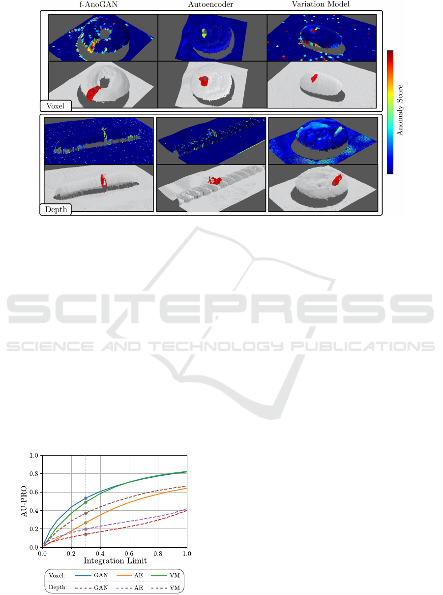
Figure 5: Qualitative anomaly localization results in which each individual method performed well. The top image visualizes

the anomaly scores as an overlay to the input point cloud. The bottom image shows the corresponding ground-truth annotation

in red. The displayed methods were only trained on the 3D data without adding color information.

Adding RGB information improves the performance

of all methods except for the Variation Models. Since

the RGB images do not contain invalid pixels, the

Depth AE and Depth f-AnoGAN beneﬁt most from

the color information. Nevertheless, the voxel-based

methods still outperform their depth-based counter-

parts. Again, Voxel f-AnoGAN shows the best overall

performance. For some object categories, however, the

Voxel AE performs better than Voxel f-AnoGAN when

including color information.

As discussed in Section 3.3, it is important to se-

lect a suitable integration limit to compute the area

under the PRO curve. To illustrate this, Figure 6 shows

the dependence of the performance of each evaluated

method on the integration limit. All methods show a

monotonic increase in their AU-PRO. When integrat-

Figure 6: Dependence of AU-PRO on the integration limit.

The results of our benchmark are reported at a limit of 0.3.

ing to a false positive rate of

, the Voxel f-AnoGAN

and the Voxel VM surpass an AU-PRO of

0.8

, which

would suggest that these methods are close to solv-

ing the task. However, evaluating at large integration

limits include binary segmentation masks where the

number of false positive predictions is extremely high.

Since the area of the defects present in our dataset

is very small compared to the area of anomaly-free

pixels, such segmentation results are no longer mean-

ingful. We found that the performance of the evaluated

methods is insufﬁcient for practical applications. We

therefore chose an integration limit of

0.3

to be able

to compare their relative performance. In the future,

we hope that our dataset sparks the development of

methods that achieve high AU-PRO scores at much

lower integration limits. In actual industrial inspec-

tion scenarios, a false positive rate of

0.3

is hardly

acceptable.

5 CONCLUSION

We presented a comprehensive 3D dataset for the task

of unsupervised detection and localization of anoma-

lies. The conceptualization and acquisition of the

dataset was inspired by real-world visual inspection

tasks. It consists of over 4000 point clouds depicting

instances of ten different object categories. The data

was acquired using a high-resolution structured light

3D sensor. About 1000 samples of the dataset con-

tain various types of anomalies and we provide precise

The MVTec 3D-AD Dataset for Unsupervised 3D Anomaly Detection and Localization

209

ground truth annotations for all of them.

We performed an initial benchmark of the few ex-

isting methods showing that there is signiﬁcant room

for improvement. In particular, the accuracy of the

evaluated methods is insufﬁcient for them to be used

in real-world industrial applications. We are convinced

that suitable datasets are a key factor in the develop-

ment of new techniques and expect our dataset to spark

the design of better methods in the future.

REFERENCES

Armeni, I., Sener, O., Zamir, A. R., Jiang, H., Brilakis, I.,

Fischer, M., and Savarese, S. (2016). 3D Semantic

Parsing of Large-Scale Indoor Spaces. In IEEE Con-

ference on Computer Vision and Pattern Recognition

(CVPR), pages 1534–1543.

Baid, U. et al. (2021). The RSNA-ASNR-MICCAI

BraTS 2021 Benchmark on Brain Tumor Segmen-

tation and Radiogenomic Classiﬁcation. Preprint:

arXiv:2107.02314.

Bakas, S., Akbari, H., Sotiras, A., Bilello, M., Rozycki,

M., Kirby, J. S., et al. (2017). Advancing the cancer

genome atlas glioma MRI collections with expert seg-

mentation labels and radiomic features. Scientiﬁc Data,

4(1).

Bengs, M., Behrendt, F., Krüger, J., Opfer, R., and Schlaefer,

A. (2021). Three-dimensional deep learning with spa-

tial erasing for unsupervised anomaly segmentation in

brain MRI. International Journal of Computer Assisted

Radiology and Surgery, 16.

Bergmann, P., Batzner, K., Fauser, M., Sattlegger, D., and

Steger, C. (2021). The MVTec Anomaly Detection

Dataset: A Comprehensive Real-World Dataset for Un-

supervised Anomaly Detection. International Journal

of Computer Vision, 129(4):1038–1059.

Bergmann, P., Fauser, M., Sattlegger, D., and Steger, C.

(2019a). MVTec AD — A Comprehensive Real-World

Dataset for Unsupervised Anomaly Detection. In IEEE

Conference on Computer Vision and Pattern Recogni-

tion (CVPR), pages 9584–9592.

Bergmann, P., Fauser, M., Sattlegger, D., and Steger,

C. (2020). Uninformed Students: Student-Teacher

Anomaly Detection With Discriminative Latent Em-

beddings. In IEEE/CVF Conference on Computer Vi-

sion and Pattern Recognition (CVPR), pages 4182–

4191.

Bergmann, P., Löwe, S., Fauser, M., Sattlegger, D., and

Steger., C. (2019b). Improving Unsupervised Defect

Segmentation by Applying Structural Similarity to Au-

toencoders. In 14th International Joint Conference

on Computer Vision, Imaging and Computer Graphics

Theory and Applications - Volume 5: VISAPP, pages

372–380. INSTICC, SciTePress.

Blum, H., Sarlin, P.-E., Nieto, J., Siegwart, R., and Ca-

dena, C. (2019). Fishyscapes: A Benchmark for Safe

Semantic Segmentation in Autonomous Driving. In

IEEE/CVF International Conference on Computer Vi-

sion Workshops (ICCVW), pages 2403–2412.

Carrera, D., Manganini, F., Boracchi, G., and Lanzarone, E.

(2017). Defect Detection in SEM Images of Nanoﬁ-

brous Materials. IEEE Transactions on Industrial In-

formatics, 13(2):551–561.

Chang, A. X., Funkhouser, T., Guibas, L., Hanrahan, P.,

Huang, Q., Li, Z., Savarese, S., Savva, M., Song, S.,

Su, H., Xiao, J., Yi, L., and Yu, F. (2015). ShapeNet:

An Information-Rich 3D Model Repository. Preprint:

arXiv:1512.03012.

Cohen, N. and Hoshen, Y. (2021). Sub-Image Anomaly De-

tection with Deep Pyramid Correspondences. Preprint:

arXiv:2005.02357.

Dai, A., Chang, A. X., Savva, M., Halber, M., Funkhouser,

T., and Nießner, M. (2017). ScanNet: Richly-

Annotated 3D Reconstructions of Indoor Scenes. In

IEEE Conference on Computer Vision and Pattern

Recognition (CVPR), pages 2432–2443.

Drost, B., Ulrich, M., Bergmann, P., Härtinger, P., and Steger,

C. (2017). Introducing MVTec ITODD — A Dataset

for 3D Object Recognition in Industry. In IEEE Inter-

national Conference on Computer Vision Workshops

(ICCVW), pages 2200–2208.

Goodfellow, I., Pouget-Abadie, J., Mirza, M., Xu, B., Warde-

Farley, D., Ozair, S., Courville, A., and Bengio, Y.

(2014). Generative Adversarial Nets. In Advances in

Neural Information Processing Systems, pages 2672–

2680.

Hoda

n, T., Sundermeyer, M., Drost, B., Labbé, Y., Brach-

mann, E., Michel, F., Rother, C., and Matas, J. (2020).

BOP Challenge 2020 on 6D Object Localization. Eu-

ropean Conference on Computer Vision Workshops

(ECCVW).

Huang, Y., Qiu, C., Guo, Y., Wang, X., and Yuan, K. (2018).

Surface Defect Saliency of Magnetic Tile. In 2018

IEEE 14th International Conference on Automation

Science and Engineering (CASE), pages 612–617.

Kingma, D. P. and Ba, J. (2015). Adam: A Method for

Stochastic Optimization. In 3rd International Confer-

ence on Learning Representations (ICLR).

Krizhevsky, A., Sutskever, I., and Hinton, G. E. (2012). Ima-

geNet Classiﬁcation with Deep Convolutional Neural

Networks. In 25th International Conference on Neu-

ral Information Processing Systems - Volume 1, pages

1097–1105.

Li, W.-X., Mahadevan, V., and Vasconcelos, N. (2013).

Anomaly Detection and Localization in Crowded

Scenes. IEEE Transactions on Pattern Analysis and

Machine Intelligence (TPAMI), 36(1):18–32.

Liew, S.-L., Anglin, J. M., Banks, N. W., et al. (2018). A

large, open source dataset of stroke anatomical brain

images and manual lesion segmentations. Scientiﬁc

data, 5:180011.

Lu, C., Shi, J., and Jia, J. (2013). Abnormal Event Detec-

tion at 150 FPS in MATLAB. In IEEE International

Conference on Computer Vision, pages 2720–2727.

Masci, J., Meier, U., Cire¸san, D., and Schmidhuber, J. (2011).

Stacked Convolutional Auto-Encoders for Hierarchi-

cal Feature Extraction. In Artiﬁcial Neural Networks

VISAPP 2022 - 17th International Conference on Computer Vision Theory and Applications

210

and Machine Learning – ICANN 2011, pages 52–59.

Springer Berlin Heidelberg.

Menze, B. H., Jakab, A., Bauer, S., Kalpathy-Cramer, J.,

Farahani, K., Kirby, J., et al. (2015). The Multi-

modal Brain Tumor Image Segmentation Benchmark

(BRATS). IEEE Transactions on Medical Imaging,

34(10):1993–2024.

Park, H., Noh, J., and Ham, B. (2020). Learning Memory-

Guided Normality for Anomaly Detection. In IEEE

Conference on Computer Vision and Pattern Recogni-

tion (CVPR), pages 14360–14369.

Salehi, M., Sadjadi, N., Baselizadeh, S., Rohban, M. H.,

and Rabiee, H. R. (2021). Multiresolution Knowledge

Distillation for Anomaly Detection. In IEEE/CVF Con-

ference on Computer Vision and Pattern Recognition

(CVPR), pages 14902–14912.

Schlegl, T., Seeböck, P., Waldstein, S., Langs, G., and

Schmidt-Erfurth, U. (2019). f-AnoGAN: Fast Unsuper-

vised Anomaly Detection with Generative Adversarial

Networks. Medical Image Analysis, 54.

Simarro Viana, J., de la Rosa, E., Vande Vyvere, T., Robben,

D., Sima, D. M., and Investigators, C.-T. P. a. (2021).

Unsupervised 3D Brain Anomaly Detection. In Brain-

lesion: Glioma, Multiple Sclerosis, Stroke and Trau-

matic Brain Injuries, pages 133–142. Springer Interna-

tional Publishing.

Song, K. and Yan, Y. (2013). A noise robust method based

on completed local binary patterns for hot-rolled steel

strip surface defects. Applied Surface Science, 285:858–

864.

Steger, C., Ulrich, M., and Wiedemann, C. (2018). Ma-

chine Vision Algorithms and Applications. Wiley-VCH,

Weinheim, 2nd edition.

Sultani, W., Chen, C., and Shah, M. (2018). Real-World

Anomaly Detection in Surveillance Videos. In IEEE

Conference on Computer Vision and Pattern Recogni-

tion (CVPR), pages 6479–6488.

Tukey, J. W. (1977). Exploratory Data Analysis. Addison-

Wesley Series in Behavioral Science. Addison-Wesley,

Reading, MA.

Ulyanov, D., Vedaldi, A., and Lempitsky, V. (2017). Im-

proved Texture Networks: Maximizing Quality and

Diversity in Feed-Forward Stylization and Texture Syn-

thesis. In IEEE Conference on Computer Vision and

Pattern Recognition (CVPR), pages 4105–4113.

Wang, S., Wu, L., Cui, L., and Shen, Y. (2021). Glancing

at the Patch: Anomaly Localization With Global and

Local Feature Comparison. In IEEE/CVF Conference

on Computer Vision and Pattern Recognition (CVPR),

pages 254–263.

Wieler, M. and Hahn, T. (2007). Weakly Supervised Learn-

ing for Industrial Optical Inspection. 29th Annual

Symposium of the German Association for Pattern

Recognition.

Wu, Z., Song, S., Khosla, A., Yu, F., Zhang, L., Tang, X.,

and Xiao, J. (2015). 3D ShapeNets: A deep repre-

sentation for volumetric shapes. In IEEE Conference

on Computer Vision and Pattern Recognition (CVPR),

pages 1912–1920.

Zeng, A., Song, S., Nießner, M., Fisher, M., Xiao, J., and

Funkhouser, T. (2017). 3DMatch: Learning Local

Geometric Descriptors from RGB-D Reconstructions.

In IEEE Conference on Computer Vision and Pattern

Recognition (CVPR), pages 199–208.

APPENDIX

Details on Training Parameters

In this section, we provide details on training pa-

rameters as well as model architectures for the deep

learning-based methods.

Voxel f-AnoGAN.

For the implementation of Voxel

f-AnoGAN, we use the same network architecture as

proposed by Simarro Viana et al. (2021). The GAN

and the encoder network are both trained for

epochs

on the augmented version of our dataset with an initial

learning rate of

0.0002

and a batch size of

using the

Adam optimizer (Kingma and Ba, 2015). The weight

for the gradient penalty loss of the GAN is set to

and one generator training iteration is performed for

every

iterations of the discriminator training. During

the training of the encoder, the “izi” and “ziz” losses

are equally weighted by choosing a loss weight of 1.

Voxel Autoencoder.

The Voxel Autoencoder con-

sists of an encoder and a decoder network. Their archi-

tecture is the same as the one of the encoder and the

generator in Voxel f-AnoGAN, respectively. We train

for

epochs on the augmented version of our dataset

with a batch size of

using the Adam optimizer with

an initial learning rate of 0.0001.

Depth f-AnoGAN.

The Depth f-AnoGAN consists

of three sub-networks, i.e., an encoder, a discrimina-

tor, and a generator. The architecture of the encoder

is given in Table 3. It consists of a stack of

con-

volution blocks that compress an input image of size

256 × 256

pixels and

channels to a

-dimensional

latent vector. Each convolution block except the last

one is followed by an instance normalization layer

(Ulyanov et al., 2017) and a LeakyReLU with slope

0.05

. The architecture of the discriminator is identical

to the one of the encoder except that

d = 1

. The gen-

erator produces an image of size

256 × 256

pixels and

channels from a latent variable with

dimensions.

Its architecture is symmetric to the one in Table 3 in

the sense that convolutions are replaced by transposed

convolution layers. Both, the GAN and the encoder

network, are trained for

epochs using a batch size of

The MVTec 3D-AD Dataset for Unsupervised 3D Anomaly Detection and Localization

211

and an initial learning rate of

0.0002

using the Adam

optimizer. During the training of the encoder, the “izi”

and “ziz” losses are equally weighted by choosing a

loss weight of 1.

Table 3: Encoder architecture of Depth f-AnoGAN and

Depth AE.

Layer Output Size Parameters

Kernel Size Stride Padding

Image 256 × 256 × c

conv1 128 × 128 × 32 4 2 1

conv2 64 × 64 × 32 4 2 1

conv3 32 × 32 × 32 4 2 1

conv4 32 × 32 × 32 3 1 1

conv5 16 × 16 × 64 4 2 1

conv6 16 × 16 × 64 3 1 1

conv7 8 × 8 × 128 4 2 1

conv8 8 × 8 × 64 3 1 1

conv9 8 × 8 × 32 3 1 1

conv10 1 × 1 × d 8 1 0

Depth Autoencoder.

For the encoder and decoder

of the Depth AE, we use the same architecture as

for the encoder and generator of Depth f-AnoGAN,

respectively. It is trained for

epochs using the Adam

optimizer at a batch size of

and an initial learning

rate of 0.0001.

Latent Dimensions of Compression-based

Methods

To select suitable latent dimensions for the evaluated

compression-based methods, we perform an ablation

study. Their mean performance over all object cat-

egories is given in Table 4. For the experiments in

Section 4, we use the respective latent dimension that

yielded the best mean performance in the ablation

study.

Table 4: Difference in performance when varying the latent

dimension of each compression-based method. We list the

area under the PRO curve up to an integration limit of

0.3

The best performing setting is highlighted in boldface.

Latent Dimension

128 512 2048

Voxel

GAN 0.536 0.583 0.555

AE 0.348 0.269 0.305

Depth

GAN 0.143 0.137 0.135

AE 0.199 0.203 0.199

Results for Anomaly Classiﬁcation

In addition to the anomaly localization results in Ta-

ble 2, we provide results for the classiﬁcation of dataset

samples as either anomalous or anomaly-free. Since

this requires a method to output a single anomaly score

for each dataset sample, we compute the maximum

anomaly score of each anomaly map. As performance

measure, we compute the area under the ROC curve.

Table 5 lists the results.

Quality of Reconstructions

For the methods based on AEs or GANs, the anomaly

detection performance signiﬁcantly depends on the

quality of their reconstructions. To get an impression

of the reconstruction quality, Figure 7 shows two ex-

amples for each evaluated method.

To visualize the voxel-based methods, voxel grids

are converted to point clouds by applying a threshold to

each cell. A cell is classiﬁed as occupied if it contains a

value of 0.9 or higher. The Voxel AE tends to produce

blurry reconstructions around the objects’ surfaces.

The Voxel f-AnoGAN does not have this problem.

However, it sometimes fails to produce parts of the

input.

For the depth-based methods, inputs and recon-

structions are visualized as depth images. Darker

shades of blue indicate points that are further from

the camera center. White points indicate invalid pixels.

Both, the Depth f-AnoGAN and the Depth AE show

problems reconstructing noisy areas that exhibit many

invalid pixels.

VISAPP 2022 - 17th International Conference on Computer Vision Theory and Applications

212

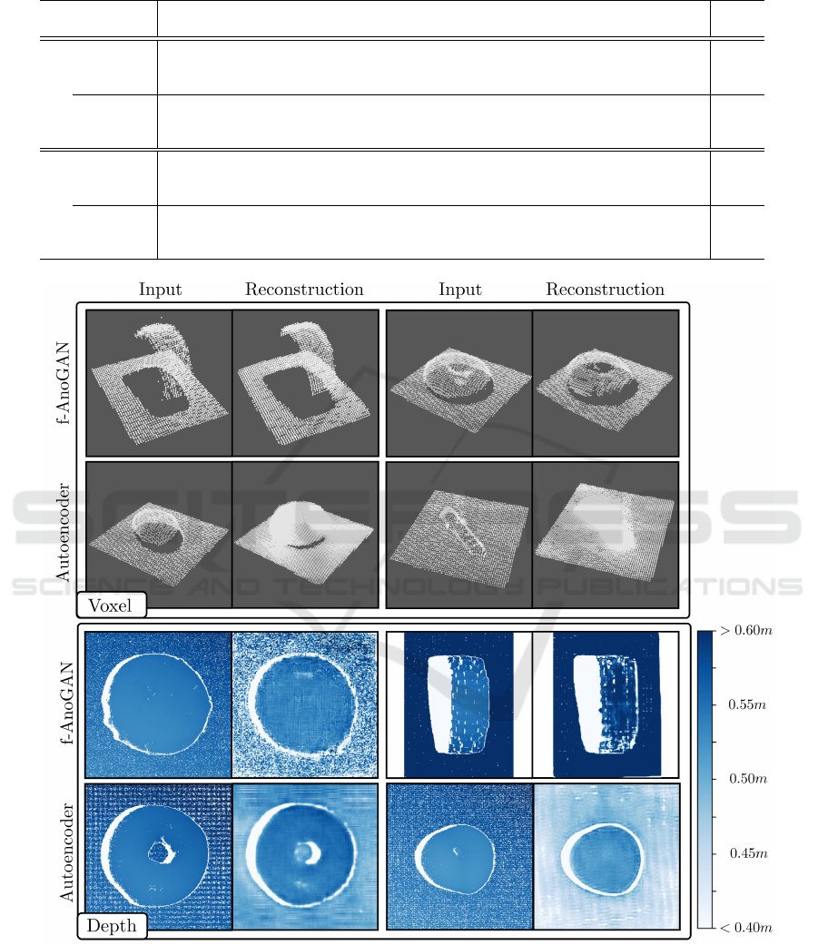
Table 5: Anomaly classiﬁcation results. We report the area under the ROC curve. The best-performing methods are highlighted

in boldface.

bagel

cable

gland

carrot cookie dowel foam peach potato rope tire mean

3D Only

Voxel

GAN 0.383 0.623 0.474 0.639 0.564 0.409 0.617 0.427 0.663 0.577 0.538

AE 0.693 0.425 0.515 0.790 0.494 0.558 0.537 0.484 0.639 0.583 0.572

VM 0.750 0.747 0.613 0.738 0.823 0.693 0.679 0.652 0.609 0.690 0.699

Depth

GAN 0.530 0.376 0.607 0.603 0.497 0.484 0.595 0.489 0.536 0.521 0.524

AE 0.468 0.731 0.497 0.673 0.534 0.417 0.485 0.549 0.564 0.546 0.546

VM 0.510 0.542 0.469 0.576 0.609 0.699 0.450 0.419 0.668 0.520 0.546

3D + RGB

Voxel

GAN 0.680 0.324 0.565 0.399 0.497 0.482 0.566 0.579 0.601 0.482 0.517

AE 0.510 0.540 0.384 0.693 0.446 0.632 0.550 0.494 0.721 0.413 0.538

VM 0.553 0.772 0.484 0.701 0.751 0.578 0.480 0.466 0.689 0.611 0.609

Depth

GAN 0.538 0.372 0.580 0.603 0.430 0.534 0.642 0.601 0.443 0.577 0.532

AE 0.648 0.502 0.650 0.488 0.805 0.522 0.712 0.529 0.540 0.552 0.595

VM 0.513 0.551 0.477 0.581 0.617 0.716 0.450 0.421 0.598 0.623 0.555

Figure 7: Examples of reconstructions for each compression-based method. For voxel-based methods, inputs and reconstructions

are visualized as point clouds. For depth-based methods, they are shown as depth images.

The MVTec 3D-AD Dataset for Unsupervised 3D Anomaly Detection and Localization

213