Storage Allocation for Camera Sensor Networks using

Feedback-based Price Discrimination

∗

Alexandre Martins

, Hung-Yu Wei

and Karl-Erik

Arz

Axis Communications and Department of Automatic Control, Lund University, Sweden

Department of Electrical Engineering, National Taiwan University, Taiwan

Department of Automatic Control, Lund University, Sweden

Keywords:

Camera Systems, Automatic Control, Resource Allocation, Price Discrimination, Video Sensors.

Abstract:

Camera sensor networks, mainly with surveillance cameras, are growing in size and complexity. Storage

space is the prime resource in such systems but current surveillance setups are still very much centralized and

limited in resources due to cost and security constraints. Allocating the correct amount of storage to each

camera sensor considering their large difference in characteristics and video content is challenging. In this

paper we propose a framework using feedback-based price discrimination of storage resources in order to

guarantee a uniform quality level of the videos in camera sensor networks, regardless of the speciﬁc camera

sensor parameters. We designed a lightweight solution using simple video quality metrics, cascade control

and PI (Proportional and Integral) controllers to deﬁne the optimal price of resources per camera.

1 INTRODUCTION

The number and size of camera sensor systems used,

e.g., in different types of public spaces with surveil-

lance cameras, are growing due to the Internet of

Things (IoT) trend and they are currently one of the

major storage and bandwidth consumers. With grow-

ing demands on high resolution, high frame rate and

level of detail, the amount of storage needed to re-

tain these videos is a growing problem. Surveillance

installations are usually critical installations and are

mostly running on dedicated infrastructures, storing

video in trusted servers owned by systems administra-

tors. Newer installations are usually large scale (com-

monly hundreds of cameras), heterogeneous and have

large differences in resource requirement. (IPVM,

2021).

In this paper we propose a lightweight solution

using the price discrimination principle from micro-

economics, (Armstrong, 2008), to allocate storage re-

sources while separating the resource providers (i.e.,

the storage units) from the resource buyers (i.e., the

camera sensors). The buyers have private information

on the amount of resources needed and act accord-

ingly to maximize their utility (here the desire to mini-

∗

This work has been partially funded by the Wallenberg

AI, Autonomous Systems and Software Program (WASP),

the ELLIIT strategic research area on IT and mobile com-

munications, and the Nordforsk university hub on Industrial

IoT (HI2OT).

mize the compression of their own video stream). The

utility represents the goal the buyers want to achieve.

The storage units enforce the constraint on resource

availability through the use of pricing.

The focus in this paper is H.264 video cam-

eras, the dominating system on the market today.

H.264 is a video compression standard based on

block-oriented, motion-compensated coding (ITU-T,

2010). A model of the bandwidth needed/generated

by a H.264 surveillance camera was presented in our

earlier work (Edpalm et al., 2018a; Edpalm et al.,

2018b). This model provides an estimate of the band-

width needs for a H.264 video given current scene

conditions and speciﬁc sensor parameters and allows

to calculate the long term resource needs for the cam-

era as long as it maintains the current parameters.

For a video surveillance system operator, the most

important metric is the video quality. As such they

want to have the best possible system-wide video

quality given the current (mostly cost) constraints

without knowledge of the prior or current character-

istics of each camera sensor. The video compression

level of H.264 videos, qp, determines the quality of

each frame. The lower the qp value, the less com-

pression is applied to the frame, the better the qual-

ity but the higher the frame size. The qp value and

its variation over time have a direct impact on the

perceived video quality (using mean opinion score

testing) according to (Xue et al., 2010; Xue et al.,

2013; Lin et al., 2012), i.e., the lower and less vary-

Martins, A., Wei, H. and Årzén, K.

Storage Allocation for Camera Sensor Networks using Feedback-based Price Discrimination.

DOI: 10.5220/0010858500003118

In Proceedings of the 11th International Conference on Sensor Networks (SENSORNETS 2022), pages 34-44

ISBN: 978-989-758-551-7; ISSN: 2184-4380

ing the compression parameter qp is, the better the

perceived quality will be. Our aim is thus to have all

video cameras in the system to deliver videos with

the same compression parameter values without hav-

ing speciﬁc information about them.

The contributions of the paper are:

• A new ﬂexible framework for facilitating resource

allocation in medium- and large-size camera sen-

sor networks.

• The use of cascade control to decide the price of

resource per camera (price discrimination) so that

the storage usage is maximized.

• A proposed utility measure for camera sensor net-

works based on the compression value (qp) and

its deviation from a nominal value.

2 RELATED WORK

Price discrimination is a known proﬁt optimization

method in economics, (Armstrong, 2008), but it has

been mostly used for revenue maximization. A study

of different pricing schemes for maximizing rev-

enue from selling cloud resources can be found in

(Xu and Li, 2013). (Li et al., 2009) studied the

maximum revenue achievable by a monopolistic ser-

vice provider under complete network information.

Revenue maximization using price discrimination for

communication network service providers was stud-

ied in (Shakkottai et al., 2008). Price discrimination

was used in order to distribute energy between sen-

sors in (Edalat et al., 2009). In (Tsakalozos et al.,

2011) the same technique was used to optimally allo-

cate virtual machines in a cloud service infrastructure.

But, to the best of the authors knowledge, however,

no prior work has used price discrimination in cam-

era sensor networks for visual quality maximization.

Some centralized bandwidth allocation techniques

optimizing the system’s compression level have been

proposed in (Seetanadi et al., 2018) and (Silvestre-

Blanes et al., 2011). Centralized task allocation for

collaborative radar sensors based on resource avail-

ability and Quality of Service are proposed in (Yan

et al., 2021) and (Giannecchini et al., 2004). An al-

ternative but related distributed approach to assign re-

sources are auctions, thus second price auctions have

been applied to video surveillance systems to opti-

mize speciﬁc applications such as area overage (Ding

et al., 2012; Konda et al., 2016; Dieber et al., 2011),

sensor placement (Elhamifar and Vidal, 2009; Ermis

et al., 2010) and object tracking (Qureshi and Ter-

zopoulos, ; Sankaranarayanan et al., ). Auction theory

has also been used to minimize content delivery delay

and caching cost for large mobile networks involving

multiple stakeholders as reported in (Li et al., 2016)

or (Ghosh et al., 2004) or to allocate tasks between

radar sensors as in (Ostwald et al., 2005).

3 ARCHITECTURE, VALUATION

& FRAMEWORK

We consider a simpliﬁed camera sensor network with

one storage unit (Network Attached Storage, Cloud

storage or other) and I IP video cameras, each having

a camera sensor, indexed with i: {C

, C

, ...C

}. An

overview of the system with I = 4 is shown in Fig-

ure 1. Typically a video surveillance camera system

is owned by a security department, which buys/rents

storage from an IT department or cloud provider

at a ﬁxed rate. In our system, viewing quality is

most important. The main system goal is to maxi-

mize the overall global video quality given the cur-

rent system constraints: running cost and video stor-

age size. The shared information between the de-

vices and the system load should be as low as pos-

sible. We therefore use the video compression fac-

tor as a computation-free and simple way to mea-

sure the video quality. The direct correlation between

the perceived video quality and the compression fac-

tor and its oscillation over time was studied in (Xue

et al., 2013) and (Xue et al., 2010). In H.264 videos,

the compression factor is deﬁned by the quantization

parameter, qp ∈ {0, 1, . . . , 51} with 0 being lossless

and 51 being the highest compression level (ITU-T,

2010). The quantization controlled by the qp value

is the only non-reversible step in the H.264 com-

pression/decompression process impacting the visual

quality.

Every predeﬁned period k, e.g., an hour, a day, or a

week, the cameras need to buy storage from the seller

to save the video they generate, using the money at

their disposal. If the cameras run out of storage they

need to wait until the next period to buy more. At

the beginning of each period, k, the cameras obtain an

amount of money, m, that they can use at their discre-

tion to buy resources. The amount they receive de-

pends on the cost of running the system. Each camera

sensor has a virtual account holding the money it may

use. Any remaining money can be saved for future

periods. The amount of money available for camera

to buy storage at the beginning of each period k is:

(k) = m

(k − 1) + m. We do not enforce a limit to

the amount of money a camera can retain if unused.

How the money is distributed and enforced is not in-

vestigated in this paper.

It is assumed that all camera sensors in the net-

Storage Allocation for Camera Sensor Networks using Feedback-based Price Discrimination

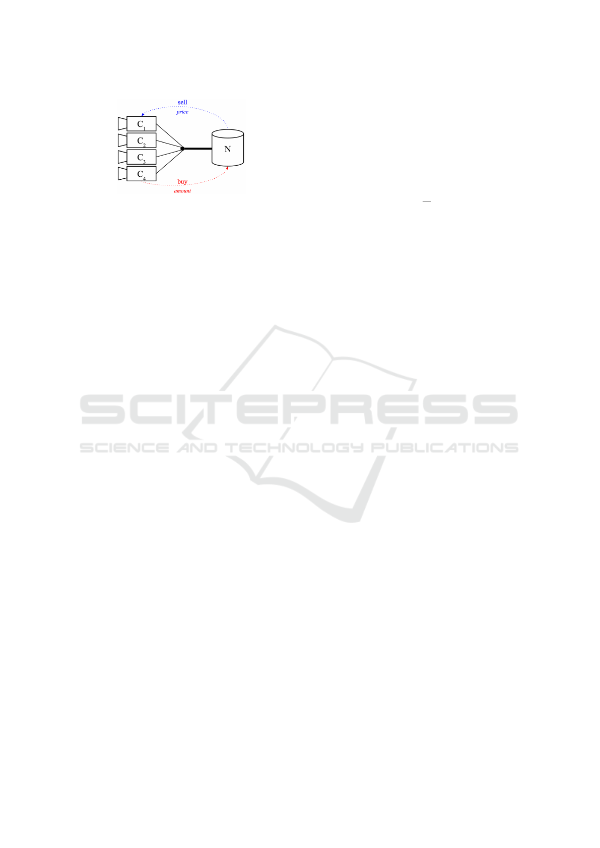
Figure 1: System with four cameras and one storage unit.

work can communicate with the seller and they could,

e.g., be part of the same virtual network. The total

quantity of storage available by the storage provider

is s and the storage space allocated to camera C

. The corresponding expected quantities are anno-

tated with a

∗

superscript, e.g. the expected allocated

storage s

to camera C

is denoted s

∗

. Only the stor-

age unit has storage space, i.e., the cameras are not

storage providers.

3.1 Price and Valuation of Resources

3.1.1 Storage Providers

The running price of each storage unit (Tbyte, Gbyte,

etc.) is determined by the storage provider. The

most common approach is to use marginal pricing,

i.e., the price is deﬁned as the running cost plus a rev-

enue margin. The storage provider will then charge

= p

min

+ ε where p

min

is the running cost and ε

the revenue margin. If p

≤ p

min

the storage provider

would sell at a loss. We can calculate p

min

from the

physical cost of hard disks, e.g., a 8Tb hard disc costs

around 400$, thus p

min

= 0.05 $ per Gb of storage.

By adding a 20% margin, we would have p

= 0, 06$.

In our approach, the seller will instead set different

(or discriminate) prices per buyer based on the quality

of the video stored by the buyer. We deﬁne the dis-

criminate price of camera i at time k as p

(k) ≥ p

min

We denote with R(k) the revenue of the seller at

time k:

R(k) =

∑

i=1

(k) · p

(k) (1)

where p

(k) is the price set by the seller and s

(k) is

the amount of storage bought by camera i at time k.

The seller wants to maximize the camera’s video

quality given the current system constraints and to ad-

just the price to reﬂect the storage limitations without

sacriﬁcing the revenue.

The compression level, i.e., qp, of H.264 videos

is part of the headers of the received videos. Hence,

in each transaction period the storage provider has ac-

cess to the qp of the received videos.

The discriminate prices are set with the help of PI

controllers (one per camera) which compute the off-

set ∆ p

(k) to the running price p

, i.e., the discrim-

inate price is p

(k) = p

+ ∆ p

(k). Proportional and

Integral (PI) control is the most widely used control

scheme in industry (Wittenmark et al., 2003). The

equation for a continuous-time PI controller is given

u(t) = K



e(t) +

e(s) ds



, (2)

where u(t) is the control signal, e(t) the error between

the desired value (or setpoint) of the measured signal

and the actual value of the measured signal, and K and

are constant parameters. The storage provider has

one controller per camera. It uses the current com-

pression level, qp, of the video as the measured sig-

nal. The setpoint is determined by a single outer-loop

probing controller which monitors the amount of stor-

age allocated. The goal of the probing controller is

to compute the desired compression level for all the

cameras so that the storage usage is maximized. Prob-

ing control is a simple version of extremum-seeking

control that is commonly used in process control, e.g.,

(Akesson and Hagander, 2000) and (Dochain et al.,

2011). The probing controller adjusts its output signal

gradually until it reaches a good enough value, prob-

ing a new value at regular intervals to check if the new

optimal value has changed.

Here the output of the probing controller is the de-

sired system compression level which is used as the

setpoint of the inner-loop PI controllers. The output

of the PI controllers, i.e., the control signal, is the dis-

criminate price offset ∆ p

(k). In order to maximize

the used storage the compression level should be as

small as possible. Hence, the probing controller will

decrease the desired compression level until the re-

quested storage is at or above the maximum storage

available. Then it will increase the desired compres-

sion level until the requested storage is within a safety

margin and then keep it constant. It is kept constant

until either (1) the requested storage is again at or

above the maximum storage available, in which case

it will start to increase the desired compression level

again, or (2) a time-out event occurs, in which case it

will again start to gradually decrease the desired com-

pression level.

The cascade architecture with n cameras is shown

in Figure 2 and the state machine of the probing con-

troller is shown in Figure 3. The sampling period of

the controllers is the transaction period and they are

executed at the beginning of each period.

The effect of the feedback-based price discrimi-

nation is that the compression levels, qp, of the cam-

eras will converge to the setpoint value of the PI con-

SENSORNETS 2022 - 11th International Conference on Sensor Networks

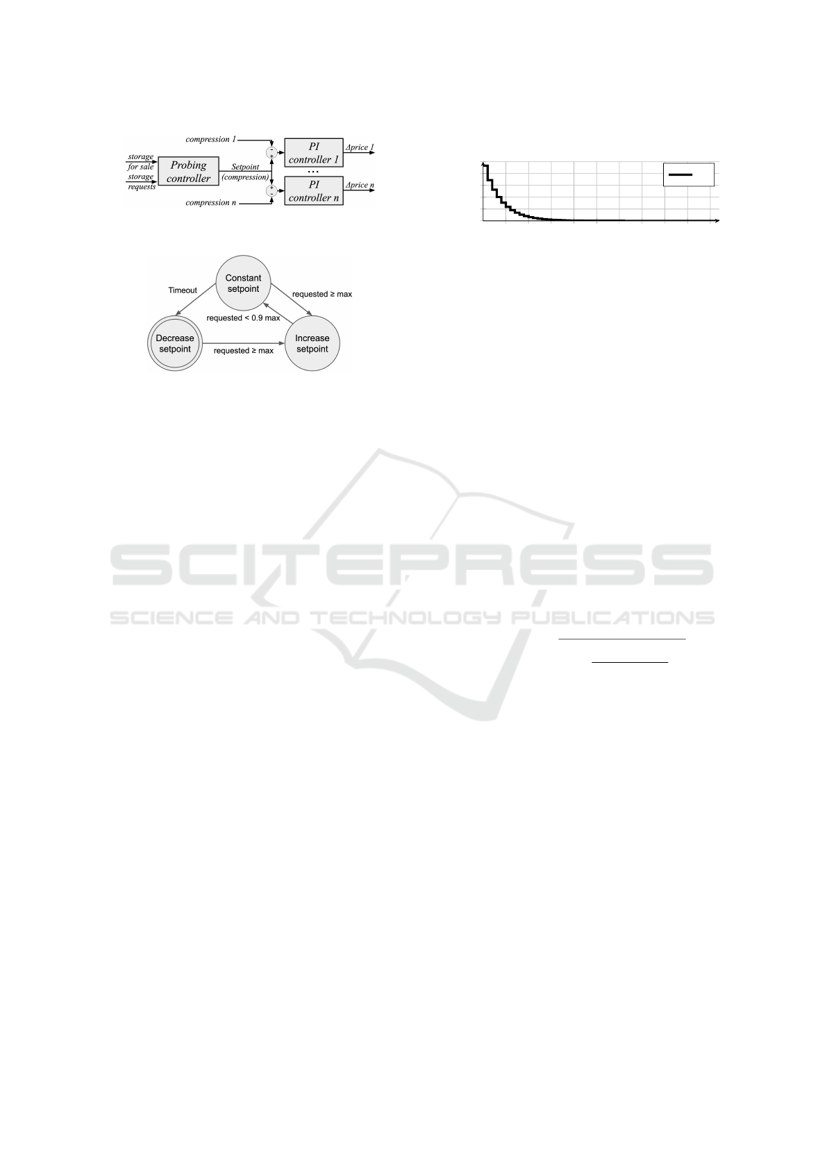
Figure 2: Cascade control structure, one probing controller

decides the setpoint of the price controllers.

Figure 3: Probing controller state machine. The double bor-

der indicates that this is the initial state. The margin avoids

rapid state changes close to the maximum storage amount.

The Timeout event occurs when the Constant setpoint state

has been active longer that a speciﬁed interval.

trollers, i.e., the value set by the outer probing con-

troller.

If the total amount of storage requested by the

cameras exceeds the total amount of available storage

for sale, the storage provide will provide each cam-

era C

with an amount of storage s

proportional to its

demand compared to that of the other cameras.

3.1.2 Cameras

In order to decide how much storage a camera C

wants to buy it needs to know how much storage it

needs to store a video of a certain quality. An esti-

mate of the storage needed for each qp is obtained us-

ing the frame size estimation model provided in (Ed-

palm et al., 2018b). This model is based on empiri-

cal values from multiple real surveillance videos. We

denote the estimated storage at the period k for cam-

era i, s

∗

i,k

(qp), it provides for each qp the expected

amount of storage necessary for a video with the cur-

rent parameters (e.g., motion in the scene, light level,

amount of nature) and settings of the speciﬁc camera

sensor (e.g., frame rate, group of picture length). An

example of s

∗

i,k

(qp) is shown in Figure 4. The higher

the qp is, the smaller the amount of storage needed

and the lower the visual quality of the video.

At the beginning of each transaction period k, each

camera C

calculates s

∗

i,k

(qp), i.e., an estimate of the

storage need for each qp ∈ {0, 1, . . . , 51} given the ac-

tual scene and camera sensor parameters which are

assumed to be measured or estimated by the cam-

era. The s

∗

i,k

(qp) functions differ from camera to cam-

era and over time because each camera sensor which

equips camera C

has different settings and overlooks

45 50

100

QP (compression)

Expected storage for different qp values

∗

Figure 4: s

∗

i,k

example.

a different non-constant scene.

Camera C

uses the actual curve to decide how

much storage it should buy with its available money

(k), see Section 3.1.3. We do not impose any lim-

itation on the saved funds of cameras and unused

money could be saved indeﬁnitely.

3.1.3 Camera Utility

The more storage the camera has, the lower qp it can

use to compress its video and therefore the better the

video quality (Xue et al., 2010) will be. Oscillations

between qp values have a large impact on the visual

quality of the video because of the visible jumps in

visual quality (Xue et al., 2013).

The valuation function θ

of buyer C

designed to

embody the system objective, i.e., to retain videos of

the highest possible quality in the system, where qual-

ity is measured by the video compression level, qp

and how much it varies. It is deﬁned by the ellipse

equation

(qp

, m

) = m

1 −



+ σ

(qp

)

2 · 51



, (3)

where m

is the money available for the camera C

, qp

the compression value corresponding to the received

amount s

, and σ

(x) is the standard deviation of x

over the n last periods.

The equation of an ellipse has an interesting char-

acteristic around its vertexes. The derivative of the

ellipse is low when approaching the co-vertex (low

qp and low σ(qp)), while it is high when close to the

vertex (high qp and high σ(qp)). It is valued more

(high derivative) to move away from the high qp and

high σ(qp) values (vertex) than it is to get closer to

the low qp and low σ(qp) values (co-vertex).

The utility u

of buyer C

is then given by

(qp

, m

, p

) = θ

(qp

, m

) − p

(4)

where p

is the price paid to obtain the amount of stor-

age s

. The smaller the compression level and the vari-

ation of the compression level the higher the camera

utility will be. An example of the utility is shown in

Fig 5. We use the last 10 qp values from previous

Storage Allocation for Camera Sensor Networks using Feedback-based Price Discrimination

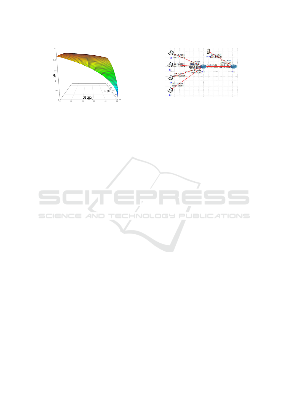
Figure 5: An illustration of how the valuation of resources,

, depends on the compression and its variation.

transactions to calculate the standard deviation. The

longer this history, the longer a deviation in qp will

affect the utility.

At the beginning of each transaction period k, af-

ter calculating the expected storage amount of storage

∗

i,k

(qp) (see Section 3.1.2), the camera calculates the

expected utility u

∗

assuming that it gets the associ-

ated storage s

∗

i,k

given the available money m

(k) and

the announced unit price p

(k).

Different cameras can have different strategies for

buying storage. Here we consider two possible strate-

gies:

1. At each period k, the camera buys the amount of

storage s

∗

i,k

which maximizes the expected utility

∗

(k) given the money m

(k) available.

2. The camera keeps all the money until an event oc-

curs. When the event occurs it acts according to

Strategy 1 (above).

3.2 Transaction Steps

We use a transaction mechanism inspired by the

closed bid transaction mechanism used in auctions

(Reck, 1997). A transaction is deﬁned by the step

described below. At the beginning of each transaction

period k:

1. Camera C

gets an amount of money, m, for the

new period k. The money available to the camera

is m

(k) = m

(k − 1) + m.

2. The storage provider, n, announces the total

amount of storage for sale, s(k), and the unit price

of camera C

: p

(k).

3. Camera C

decides how much it buys based on the

expected storage usage s

∗

i,k

(qp), p

(k) and m

(k).

It sends to n the amount from s

∗

i,k

(qp) maximizing

its expected utility u

∗

(k) (see Section 3.1.3).

4. Storage provider n decides the storage allocation

and sends to C

the amount of storage it is allowed

to buy, s

Figure 6: CORE network emulator setup.

5. Camera C

pays the storage provider n the price

· p

, deduces this amount from the money it has,

i.e., m

(k) = m

(k) − s

· p

, and starts streaming

video data up to the provided amount s

allocated.

6. Storage n extracts the compression level from the

received videos, qp

(k), and uses it to decide the

price for the next transaction p

(k + 1) using the

PI controllers. It also calculates the total amount

of storage allocated,

∑

(k), and uses it to adjust

the desired compression level using the probing

controller so that the storage usage is maximized,

see 3.1.1.

4 RESULTS

To validate the price discrimination approach we run

multiple simulations using a python framework with

independent players (seller and buyers) communicat-

ing via queues as well as simulations using the CORE

real time network emulator (Ahrenholz et al., 2008).

Each simulation uses random unit prices, p

, and ran-

dom camera parameters (resolution and motion level).

The storage needs of the cameras are determined us-

ing the model described in (Edpalm et al., 2018b).

The cameras will have a computation horizon of 10

periods to calculate their utility.

In the simulations we compare three different

cases:

1. The storage uses marginal pricing, i.e., it deﬁnes

the running cost and adds a margin to it (see Sec-

tion 3.1.1).

2. The storage uses the price discrimination scheme

described in Section 3 with a ﬁxed system quality

setpoint, i.e., without any probing controller.

3. The storage uses the price discrimination scheme

described in Section 3 with the probing controller

selecting the system quality setpoint.

The camera utility is given by Equation (4). We

also deﬁne a seller utility U(k) to visualise how ef-

ﬁciently the proposed approach reduces the standard

SENSORNETS 2022 - 11th International Conference on Sensor Networks

deviation of the sum of the compression levels. It is

given by

U (k) =



∑

(k)



(5)

The simulations use four cameras in Fig 7 and Fig-

ure 9 and ten cameras in Figure 8. The storage price

is set randomly at simulation start. In the simula-

tions in Figure 7 and Figure 9, C

is a 4K camera and

as such requires the largest storage amount, C

and C

are 1080p cameras with different scene characteristics

’s video is more noisy and has more motion) and

is a 720p camera. In Figure 8, camera parameters

are randomly selected at simulation start. During the

simulations the camera parameters are constant (reso-

lution and motion levels are ﬁxed) but uniform noise

of amplitude up to 25% of the frame sizes was added

to reﬂect a real scenario where noise from the sensor

and small changes in the scene would create changing

frame sizes. All cameras receive the same amount of

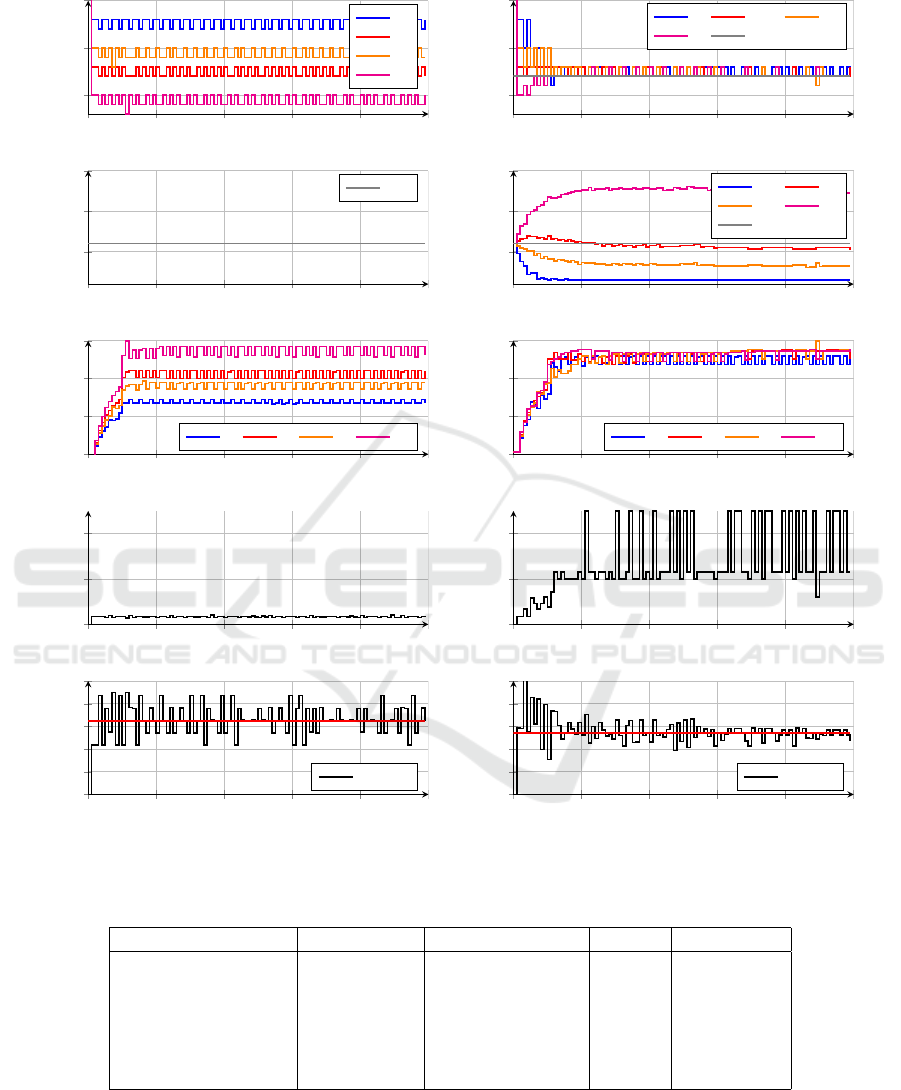
money m at each period k. Figure 7 shows the sim-

ulation results of case 1 and case 2. The left column

contains the results using marginal pricing scenario

(case 1) and the right column contain the results us-

ing price discrimination with PI control but without

probing controller, i.e., with a ﬁxed setpoint (case 2).

The uppermost plots contain the qp values of the

cameras (remember that a higher qp means a lower

video quality), the ones below are the prices set by

the storage provider (gray for the base price, colored

for discriminate prices). The third row is the camera

utility and the ﬁnal two rows show the seller utility

(deﬁned in 1) and the revenue from selling storage to

the cameras (see 3.1.1). Note that in the utility plots

the maximum utility has been limited to 5 for easier

plotting and calculations (as the utility of an inﬁnites-

imal standard deviation tends to inﬁnity).

In the right column of Figure 7, we can see that the

PI controllers change the unit prices p

to allow the

video compression qp

to converge towards a com-

mon qp value (ﬁrst row). The seller utility U (fourth

row) in the price discrimination case (case 2, right

column) is clearly higher than in the ﬁxed price case

(case 1, left column) while the seller revenues R are

very close to each other (ﬁfth row), i.e., the price dis-

crimination policy allows the total system to run in

a better state than using marginal price policy. Be-

cause of the seller utility deﬁnition, the utility value

will tend to inﬁnity when the standard deviation of

the camera qp is zero, leading to the jumps we can

see in Figure 7.

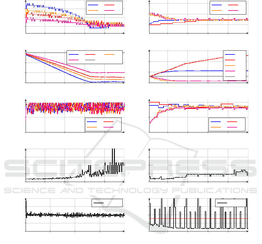
In the simulations in Figure 9 price discrimina-

tion with probing controller (case 3) is used in both

columns. The camera parameters (apart for the video

resolution) are selected randomly at simulation start.

The results in the left and right column are from two

different runs. In the left column, cameras are buy-

ing storage at each period k, the simulation being run

for 400 periods. In the right column the simulation

is done with 4 cameras over 100 periods, cameras C

and C

are buying at each time period but C

and C

only buy every 5 and 12 periods respectively. The

simulations were done using the same code and mod-

els as the python framework but the seller and buy-

ers were running in virtual machines communicat-

ing through sockets in the CORE real time network

emulator (Ahrenholz et al., 2008). A screenshot of

the used system can be seen in Figure 6. With the

CORE simulator we can simulate multiple machines

communicating over different network architectures

and simulate different network conditions. We used

the CORE simulator to ensure communication was

not sequential and reﬂected a real-world setup with-

out having to deploy such a setup. The focus of the

python framework is to simulate the system sequen-

tially with a focus on the global system behavior.

In the right part of Figure 9 the seller revenues os-

cillate because of the less frequent storage buy from

cameras C

and C

, but the average revenue is com-

parable and the different strategies does not prevent

the system from converging to a common compres-

sion level. In the left part of Figure 9, we can observe

the effect of the probing controller adjusting gradu-

ally the setpoint compression level down in order to

maximize the storage usage, leading to a stable sys-

tem value with qp = 20. We can also see that the

prices set follows the same trend in order to converge

to the system setpoint set by the probing controller but

also each discriminate prices diverge in order for the

compression of each camera to converge to a common

value thanks to the price discrimination PI controllers.

Figure 8 shows simulations with 10 cameras and

same selected parameters (randomly chosen once for

both simulations) and we visualize the most interest-

ing 250 periods. In this ﬁgure, the left side has only

the price discrimination PI controllers (case 2) run-

ning with a manually ﬁxed global quality setpoint of

qp = 25 (which is the optimal setpoint for this spe-

ciﬁc system). The right side of the ﬁgure shows the

same parameters with the setpoint controller (case

3) converging autonomously to the optimal value of

qp = 25. In the left column (case 2) we can see that

all cameras converge slowly to the deﬁned setpoint

while on the right (case 3) they converge faster and

autonomously to the desired quality levels.

Finally, to test the robustness of the proposed ap-

proach, we run 100 simulations of 500 transactions

period k each with price discrimination (case 3) and

100 others with marginal pricing (case 1) where all

Storage Allocation for Camera Sensor Networks using Feedback-based Price Discrimination

QP values per transactions

Target

Price per transactions

Base

Price per transactions

Base

0.4

0.6

0.8

Cameras utilities

0.4

0.6

0.8

Cameras utilities

Storage utility

0 20 40

80 100

Storage revenue

Average R

0 20 40

80 100

Storage revenue

Average R

Figure 7: Fixed price (left) and discriminate price (right) with ﬁxed system setpoint (no probing controller) for 4 cameras.

Table 1: Multiple simulations results.

Discriminate Discriminate+rnd Margin Margin+rnd

Seller utilities mean 1.68 0.56 0.33 0.27

Seller revenue mean 19.8 20 20 20

Buyer 1 utility mean 0.87 0.82 0.81 0.78

Buyer 2 utility mean 0.86 0.82 0.8 0.75

Buyer 3 utility mean 0.86 0.82 0.83 0.79

Buyer 4 utility mean 0.86 0.83 0.82 0.8

cameras were buying at each period k. We also run

simulations with random uniform distributed video

parameters changing from frame to frame. In real-

ity this is highly unlikely to happen, but demonstrate

a hypothetical worst case scenario. This is denoted

with ”+rnd” in Table 1.

A global summary of the simulation runs can be

found in Table 1. The seller utilities U are on average

SENSORNETS 2022 - 11th International Conference on Sensor Networks

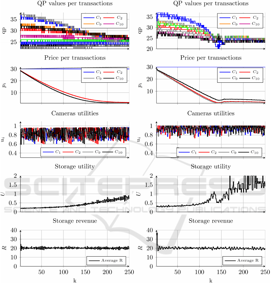
Figure 8: Discriminate price with ﬁxed setpoint (left) and with probing controller (right) for 10 cameras.

(mean) higher in the discriminate pricing (1.68 and

0.56) than for the marginal pricing (0.33 and 0.27).

Note that the utility difference between the random

and non-random case in Table. 1 comes from the util-

ity being based on σ

(qp). With randomly chang-

ing video parameters, the optimal qp value will rarely

stay equal to the system setpoint qp value, thus lead-

ing to a lower utility value for the storage than in a

more stable environment. The revenue R remains very

close at 19.8 and 20 for the discriminate pricing ver-

sus 20 for the margin pricing indicating no noticeable

loss in revenue for the seller. The buyer utilities u

have higher values with price discrimination than with

the marginal pricing because of the visual quality uni-

formity enforced by the storage provider.

5 CONCLUSIONS & FUTURE

WORK

In this work we proposed a method based on price

discrimination of storage costs for system-level op-

Storage Allocation for Camera Sensor Networks using Feedback-based Price Discrimination

QP values per transactions

Price per transactions

Base

Price per transactions

Base

0.5

Cameras utilities

0.5

Cameras utilities

Storage utility

100 200 300 400

Storage revenue

Average R

20 40

80 100

Storage revenue

Average R

Figure 9: Discriminate price with setpoint probing controller for continuous buyers only (left) or continuous and event buyers

(right) for 4 cameras.

timization of video quality, which to the best of the

authors knowledge is a novel approach to solve video

storage allocation. The approach is lightweight and

requires limited system knowledge and computation

requirements. The results in terms of system-wide

video quality are encouraging and do not lead to sig-

niﬁcant revenue loss for the storage sellers but im-

proves the overall system video quality. The simpli-

ﬁed approach also lays the ground for future develop-

ment of game theory approaches using the same trans-

action framework.

A logical extension of this paper would be to han-

dle multiple storage providers and develop more com-

plex utility functions for both cameras and storage

sellers which would take into account different con-

straints such as network latency and bandwidth. We

could also use a different convergence method which

would optimize the storage usage more by allowing

the compression levels to slightly deviate for some

cameras. Instead of having the probing controller in-

creasing or decreasing the compression level for all

the cameras it could increase/decrease the compres-

sion level of the cameras one at a time, ensuring that

SENSORNETS 2022 - 11th International Conference on Sensor Networks

at all times the cameras have setpoints that maximally

differ with one compression level value. This would

increase the storage utilization.

A limitation of this work is that we expect the stor-

age provider to be able to access the received videos

in order to get access to the qp values in order to de-

cide on a discriminate price. If the video is stored in

an encrypted format this technique could not be used.

Video quality is here considered as correlated to the

video compression. An alternative approach would be

to use an application speciﬁc metric or a recognized

quality metric such as the structural similarity index

measure (SSIM), peak signal-to-noise ratio (PSNR)

or other metrics enumerated in (Yang, 2007), but at

the expense of additional computation costs.

REFERENCES

Ahrenholz, J., Danilov, C., Henderson, T. R., and Kim,

J. H. (2008). Core: A real-time network emulator. In

MILCOM 2008-2008 IEEE Military Communications

Conference, pages 1–7. IEEE.

Akesson, M. and Hagander, P. (2000). A simpliﬁed prob-

ing controller for glucose feeding in escherichia coli

cultivations. In Proceedings of the 39th IEEE Confer-

ence on Decision and Control (Cat. No.00CH37187),

volume 5, pages 4520–4525 vol.5.

Armstrong, M. (2008). Price discrimination. MIT Press.

Bernhard Dieber, Christian Micheloni, and Bernhard Rin-

ner. ”Resource-aware coverage and task assignment

in visual sensor networks”. In: IEEE Transactions

on Circuits and Systems for Video Technology 21.10

(2011), pp. 1424–1437.

Chong Ding et al. ”Collaborative Sensing in a Distributed

PTZ Camera Network”. In: IEEE Transactions on

Image Processing 21 (July 2012), pp. 3282–3295.

Dochain, D., Perrier, M., and Guay, M. (2011). Extremum

seeking control and its application to process and re-

action systems: A survey. Mathematics and Comput-

ers in Simulation, 82(3):369–380. 6th Vienna Interna-

tional Conference on Mathematical Modelling.

Edalat, N., Xiao, W., Tham, C.-K., Keikha, E., and Ong,

L.-L. (2009). A price-based adaptive task allocation

for wireless sensor network. In 2009 IEEE 6th In-

ternational Conference on Mobile Adhoc and Sensor

Systems.

Edpalm, V., Martins, A.,

Arz

en, K.-E., and Maggio, M.

(2018a). Camera networks dimensioning and schedul-

ing with quasi worst-case transmission time.

Edpalm, V., Martins, A., Maggio, M., and

Arz

en, K.-E.

(2018b). H.264 Video Frame Size Estimation.

Ehsan Elhamifar and Ren Vidal. ”Distributed calibra-

tion of camera sensor networks”. In: 2009 3rd

ACM/IEEE Int. Conference on Distributed Smart

Cameras, ICDSC 2009 (2009).

Erhan Baki Ermis et al. ”Activity based matching in dis-

tributed camera networks”. In: IEEE Transactions on

Image Processing

Ghosh, P., Roy, N., Das, S. K., and Basu, K. (2004). A

game theory based pricing strategy for job allocation

in mobile grids. In 18th Int. Parallel and Distributed

Processing Symp., 2004. Proceedings., pages 82–.

Giannecchini, S., Caccamo, M., and Shih, C.-S. (2004).

Collaborative resource allocation in wireless sensor

networks. In Proceedings. 16th Euromicro Confer-

ence on Real-Time Systems, 2004. ECRTS 2004.

IPVM. Top 5 Problems in Video Surveillance Stor-

age. url: https://ipvm.com/reports/problems-video-

surveillance-storage (visited on 08/18/2021).

ITU-T (2010). H.264 standard documentation.

Krishna Reddy Konda, Nicola Conci, and Frnacesco De

Natale. ”Global coverage maximization in PTZ cam-

era networks based on visual quality assessment”. In:

IEEE Sensors Journal (2016).

Li, J., Sun, J., Qian, Y., Shu, F., Xiao, M., and Xiang,

W. (2016). A commercial video-caching system for

small-cell cellular networks using game theory. IEEE

Access, 4:7519–7531.

Li, S., Huang, J., and Li, S.-Y. R. (2009). Revenue max-

imization for communication networks with usage-

based pricing. In GLOBECOM 2009-2009 IEEE

Global Telecommunications Conference, pages 1–6.

IEEE.

Lin, X., Ma, H., Luo, L., and Chen, Y. (2012). No-

reference video quality assessment in the compressed

domain. IEEE Transactions on Consumer Electronics,

58(2):505–512.

Ostwald, J., Lesser, V., and Abdallah, S. (2005). Combina-

torial auctions for resource allocation in a distributed

sensor network. In 26th IEEE International Real-Time

Systems Symposium (RTSS’05).

Qureshi, F. Z. and Terzopoulos, D. In 2009 Third

ACM/IEEE Int. Conference on Distributed Smart

Cameras (ICDSC).

Reck, M. (1997). Trading-process characteristics of elec-

tronic auctions. Electronic Markets, 7(4):17–23.

Sankaranarayanan, A., Veeraraghavan, A., and Chellappa,

Seetanadi, G. N., Oliveira, L., Almeida, L., Arz

en, K.-

E., and Maggio, M. (2018). Game-theoretic network

bandwidth distribution for self-adaptive cameras.

Shakkottai, S., Srikant, R., Ozdaglar, A., and Acemoglu,

D. (2008). The price of simplicity. IEEE Journal on

Selected Areas in Communications, 26(7):1269–1276.

Silvestre-Blanes, J., Almeida, L., Marau, R., and Pedreiras,

P. (2011). Online qos management for multimedia

real-time transmission in industrial networks. IEEE

Transactions on Industrial Electronics, 58(3):1061–

1071.

Tsakalozos, K., Kllapi, H., Sitaridi, E., Roussopoulos, M.,

Paparas, D., and Delis, A. (2011). Flexible use of

cloud resources through proﬁt maximization and price

discrimination. In 2011 IEEE 27th International Con-

ference on Data Engineering, pages 75–86. IEEE.

Wittenmark, B.,

Astr

om, K., and

Arz

en, K.-E. (2003).

Computer control: An overview. Technical report, De-

partment of Automatic Control, Lund University.

Storage Allocation for Camera Sensor Networks using Feedback-based Price Discrimination

Xu, H. and Li, B. (2013). A study of pricing for cloud re-

sources. ACM SIGMETRICS Performance Evaluation

Review, 40(4):3–12.

Xue, Y., Ou, Y.-F., Ma, Z., and Wang, Y. (2010). Perceptual

video quality assessment on a mobile platform con-

sidering both spatial resolution and quantization arti-

facts. In 2010 18th International Packet Video Work-

shop, pages 201–208. IEEE.

Xue, Y., Song, Y., Ou, Y.-F., and Wang, Y. (2013). Video

adaptation considering the impact of temporal varia-

tion on quantization stepsize and frame rate on per-

ceptual quality. In International workshop on video

processing and quality metrics for consumer electron-

ics, pages 70–74.

Yan, J., Dai, J., Pu, W., Zhou, S., Liu, H., and Bao, Z.

(2021). Quality of service constrained-resource al-

location scheme for multiple target tracking in radar

sensor network. IEEE Systems Journal.

Yang, K.-C. (2007). Perceptual quality assessment for com-

pressed video. PhD thesis, UC San Diego.

SENSORNETS 2022 - 11th International Conference on Sensor Networks