Types of Flexible Job Shop Scheduling: A Constraint Programming

Experiment

Erich C. Teppan

1,2 a

Universit

at Klagenfurt, Austria

Fraunhofer Austria - KI4Life, Austria

Keywords:

Flexible Job Shop Scheduling, Constraint Programming, Empirical Evaluation.

Abstract:

The scheduling of jobs is a crucial task in every production company and becomes more and more important

in the light of the fourth industrial revolution (Industry 4.0) that aims at fully automated processes. One

such problem formulation with big practical relevance is the ﬂexible job shop scheduling problem (FJSSP).

Since the classic problem formulation is more general than what can be found in most of nowadays industrial

environments, this paper introduces different types of ﬂexibility and investigates how the ﬂexibility type, the

amount of allowed ﬂexibility and the presence of machine dependent processing times inﬂuence the solution

quality that can be achieved by a state-of-the-art constraint solver within limited time. Results show that

certain forms of ﬂexibility, higher ﬂexibility factors and the absence of machine dependent processing times

can ease the problem.

1 INTRODUCTION

Scheduling and particularly the scheduling of jobs

(Blazewicz et al., 2014) has been an active ﬁeld of re-

search at least since the mid of the last century (Muth

and Thompson, 1963; Johnson, 1953; Manne, 1960;

Bowman, 1959). In the industrial context schedul-

ing has become more important than ever in the light

of Industry 4.0 (also sometimes called the fourth in-

dustrial revolution) which aims at full automation and

digitization of processes, in particular production pro-

cesses (Lasi et al., 2014). Among the various deﬁni-

tions of different scheduling problems the ﬂow shop

scheduling problem (FSSP) (Johnson, 1953) and the

job shop scheduling problem (JSSP) (Brucker and

Schlie, 1990; Brucker and Jurisch, 1993; Applegate

and Cook, 1991) play an especially important role for

production plants. Both, FSSP and JSSP, are known

to be NP-hard problems (Garey et al., 1976).

Informally spoken, the problems can be described

as follows: In FSSP and JSSP a set of jobs is to be

accomplished by a set of machines (or resources in

general). A job can be thought of as the production

process carried out to create a certain product. This

process, i.e. the job, is sub-divided into job operations

each of which has to be performed by a dedicated ma-

chine and possesses a predetermined processing time

https://orcid.org/0000-0001-8397-9303

on the assigned machine (preemption is not allowed).

Hence, the machine and the corresponding process-

ing time for each job is part of the input. The prob-

lem consists in ordering the job operations on each

machine such that some optimization criterion is opti-

mized, e.g. minimization of the total completion time.

What makes the FSSP different from the JSSP is that

the order in which jobs go through the different ma-

chines is the same for all jobs (though the processing

times can vary). Take as an explanatory example for

a FSSP a bakery. In principle, every bread has to go

through the same production steps in the same order

although recipes and related processing times differ

for different products. In the JSSP, the order in which

jobs go through the machines differ between jobs. Ex-

amples for that can be found in factories where dif-

ferent types of products are produced (e.g. for some

products the cutting operation might be before the

screwing operation and for other products it might be

the other way round). Thus, the FSSP can be seen as a

special of the JSSP. For the classic JSSP (and as well

for the FSSP) for each operation there exists only one

possible machine which can/must execute it. Thus,

there is no guessing about operation-to-machine as-

signments. However, for many real scenarios these

assumptions are to restrictive.

The ﬂexible job shop scheduling problem (FJSSP)

(Chaudhry and Khan, 2015) is a direct generalization

516

Teppan, E.

Types of Flexible Job Shop Scheduling: A Constraint Programming Experiment.

DOI: 10.5220/0010849900003116

In Proceedings of the 14th International Conference on Agents and Artiﬁcial Intelligence (ICAART 2022) - Volume 3, pages 516-523

ISBN: 978-989-758-547-0; ISSN: 2184-433X

of the JSSP allowing more than one machine for a job

operation, also with different processing times for the

same operation. This introduces the routing problem,

hence, the assignment of job operations to machines

is not predetermined and is part of the solution and

not part of the input as for the JSSP. Although, the

JSSP as well as the FJSSP are NP-hard and their deci-

sion problem versions

are NP-complete, the FJSSP is

widely assumed to be generally harder than the JSSP

because of the additional routing sub-problem. This

view is supported by the fact that by increasing the

ﬂexibility (i.e. more than one machine could perform

a job operation) also the number of possible (though

not forcibly optimal) schedule solutions is increased

at the same time. Consequently, the search space for

an optimal schedule is bigger.

However, from a practical point of view, some as-

pects could ease the problem signiﬁcantly:

1. First of all, for many application areas there are

not (signiﬁcantly) different processing times for

the same operation on different machines. Take

as a simple example the bakery described above.

How long an operation takes is dependent on the

type of bread but not on the type of the oven.

2. A second important point where the FJSSP allows

more generality than needed for many application

areas is that in the FJSSP there are no restrictions

on which machines can perform the same oper-

ations and as a matter of fact typical benchmark

problems use totally random machine sets. In real

application scenarios, though, the reason why a

certain amount of ﬂexibility for machine assign-

ment is possible is that machines are similar or

equal. As a consequence, they can execute the

same set of operations and, thus, implement par-

allelism.

3. A third issue that is not taken into account when

stating that the FJSSP is harder than the JSSP is

the question of optimality. It is rather intuitive

that in the worst case to ﬁnd an optimal solu-

tion for a FJSSP is harder than for a JSSP due

to the bigger search space. However, most of-

ten in real application environments absolute op-

timality is not needed and near-optimal solutions

are enough. The bigger search space should also

increase the number of good enough solutions so

that it is not clear whether higher ﬂexibility fac-

tors really increase hardness when searching only

a near-optimal solution.

Deciding whether there exists a solution with an ob-

jective value equal or better than some given constant (e.g.

completion time ≤ κ).

In this paper we try to identify easier classes of

FJSSP from a practical constraint solving point of

view. To this end, we introduce different types of

ﬂexibility and report on an experiment based on prob-

lem instances derived from a large scale JSSP bench-

mark suite (Da Col and Teppan, 2021) where we sys-

tematically change ﬂexibility factors, types of ﬂexi-

bility and whether processing times are machine de-

pendent or not. For solving the problem instances

we use constraint programming (CP) out of three rea-

sons: First of all, CP has a long and successful history

in solving job scheduling problems (Fox et al., 1982;

Fox et al., 1989; Sycara et al., 1991; Sadeh and Fox,

1996; Keng and Yun, 1989; Rodler et al., 2021). Sec-

ond, CP solvers are currently the strongest for solving

scheduling problems, with IBM’s CP Optimizer and

Google’s OR Tools leading the way (Laborie et al.,

2018; Da Col and Teppan, 2019a; Da Col and Tep-

pan, 2019b). The third important reason is that in CP

it is possible to give a worst case estimation on how

far some current best solution is off the optimum since

lower and upper bounds are inherently calculated by

constraint propagation techniques. This is crucial for

many real life problems for which optimal solutions

are generally out of reach.

The further reading is as follows: In Section 2 we

formally deﬁne the FJSSP and some special ﬂexibility

types that are sufﬁcient for many real life application

scenarios. In Section 3 we discuss a state-of-the-art

constraint model to be used with IBM’s CP Optimizer.

In Section 4 we present an empirical evaluation that

analyzes the impact different types of ﬂexibility, the

amount of allowed ﬂexibility and machine dependent

processing times have on the proven quality of (near-

) optimal solutions found within limited calculation

time.

2 THE FLEXIBLE JOB SHOP

SCHEDULING PROBLEM

The ﬂexible job shop scheduling problem (FJSSP)

can be deﬁned as follows:

Deﬁnition 1. Given a set of machines M =

, . . . , m

} and a set of jobs J = { j

, . . . , j

(1) Each job j ∈ J consists of a sequence of opera-

tions O

= { j

, . . . , j

} whereby j

is the last op-

eration of job j.

• For a job j and its operation j

, the operation

i+1

is called successor, and the operation j

i−1

is called predecessor.

• We refer to the set of all operations as

O =

j∈J

Types of Flexible Job Shop Scheduling: A Constraint Programming Experiment

517

(2) For each operation o, there is a non-empty set of

machines M

⊆ M representing the machines that

are able (or allowed) to process operation o.

• We refer to the maximum size of the operations’

machine sets max{|M

| : o ∈ O} as the prob-

lem’s ﬂexibility factor f lex.

(3) For each operation o ∈ O and machine m ∈ M

there is a predeﬁned processing time time

o,m

∈ N.

(4) A (consistent and complete) schedule consists of

an assigned machine m

∈ M

and a start time

start

∈ N for each operation o ∈ O such that:

• An operation’s successor starts only after the

operation is ﬁnished:

start

i+1

≥ start

+ time

• Operations on the same machine do not over-

lap:

start

≤ start

−→ start

+ time

o1,m

≤

start

(5) An objective function is optimized.

• One of the most classic optimization criteria in

this context is the completion time C

max

, that is

the time span needed for processing all opera-

tions:

minimize max{start

+ time

o,m

: o ∈ O}

The FJSSP is strongly NP-hard. Already the job

shop scheduling problem (JSSP), being a special case,

is strongly NP-hard (Garey et al., 1976). As in the

JSSP for each operation there exists only one machine

that can process it, the JSSP can be seen as a FJSSP

with ﬂexibility factor f lex = 1.

Observation 1. Deﬁnition 1 (2) does not specify

how machine sets M

⊆ M are composed and why.

In real production environments operations and ma-

chines are tied together via the concept of operation

types. Each operation o possesses a type t

∈ T and

a machine m supports one or more operation types

⊆ T . A machine m can process an operation o if

(and only if) t

∈ T

Depending on the actual production line layout

and machine capabilities, the concept of operation

types offers the possibility of identifying different

types of ﬂexibility that can be present and we expect

this to have a signiﬁcant impact on the hardness of a

FJSSP.

Observation 2. In many cases, the processing times

for a certain operation is the same for every machine

that can process it (or differences are small and can

be neglected). Consequently, there would be only one

machine independent processing time (time

) for each

operation o instead of machine dependent processing

times (time

o,m

, compare Deﬁnition 1 (3)).

With respect to Observation 1 we introduce three

special types of ﬂexibility in job shops, which can

be found in nowadays industrial production environ-

ments (see Figure 1).

Imagine a classic job shop, i.e. a production envi-

ronment with exactly one machine for each operation

type (Figure 1-a). Now it is possible to ﬂexibilize this

job shop by adding new machines such that multiple

machines operate in parallel for the same operation

type (Figure 1-b). In this case, although the number of

possible machines for an operation type increases, the

number of operation types a machine supports does

not increase.

Another common shop conﬁguration that can be

found are closed machine sets (Figure 1-c). In this

case, machines support multiple operation types and

can be sub divided into closed subsets containing ma-

chines with the same capabilities.

Another shop conﬁguration is given when multi

purpose machines have asymmetric capabilities, thus

do not form closed machine sets, yet are linked by

their capabilities (Figure 1-d). In the most extreme

case this forms a chain where there is a machine that

supports type A and B, the second machine supports

type B and C, the third type C and D and so on.

All of those different FJSSPs remain NP-hard as

they all contain the classic JSSP as a special case that

is strongly NP-hard itself. The basic question treated

in this paper is how increased ﬂexibility factors, the

ﬂexibility type (see Figure 1) and machine dependent

processing times (see Observation 2) inﬂuence the

hardness of the FJSSP (in particular for CP solvers

as they are currently the means of choice for job shop

scheduling problems).

3 CP MODEL

A state-of-the-art CP model for the FJSSP expressed

in IBM’s modelling language OPL

is depicted in

Listing 1.

1usi n g CP ;

3tup l e pa r amsT {

4int nb J ob s ; int nb M ch s ;

5};

7tup l e O p er ati o n {

8int opId ; i n t jobI d ; in t p o s ;

9};

11tup l e Mode {

12int opId ; i n t m c h ; in t pt ;

https://www.ibm.com/docs/en/icos/20.1.0?topic=opl-

optimization-programming-language

ICAART 2022 - 14th International Conference on Agents and Artiﬁcial Intelligence

518

Figure 1: Different types of ﬂexibility in job shops with ﬂexibility factor f lex = 2.

13};

15pa r am sT Pa r a ms = . . .;

16{ Op er ati o n } Ops = . . .;

17{ Mode } Mod e s = . . . ;

19ran g e Jobs = 1.. Par a ms . n bJ ob s ;

20ran g e Mchs = 1.. Par a ms . n bM ch s ;

22i n t j la st [ j in J o b s ] = max (o in Ops :

o . j o bI d == j) o . pos ;

24d va r in t er val ops [ O p s ] ;

25d va r in t er val m od e s [md in M o d es ]

op t io nal s i ze md . pt ;

26d va r se q ue nce m c hs [ m in Mc h s ] in

all ( md in M od e s : md . mc h == m )

mod e s [ md ];

28mi n imi z e ma x ( j in Jobs , o in Ops :

o . pos == j l as t [ j ] ) e n dO f ( ops [ o ]) ;

30su b je ct to {

31f o r al l ( o in Ops )

32al t ern at ive ( ops [ o ], a l l ( md in

Mod e s : md . opId == o. opId ) mode s [ md ]) ;

33f o r al l ( m in Mc h s )

34no O ver l ap ( mchs [ m ]) ;

35f o r al l ( j in Jobs , o1 in Ops , o2 in

Ops : o1 . jo b I d == j && o2 . jobI d == j

36&& o2 . po s ==1+ o 1 . po s )

en dBe f ore Sta r t ( ops [ o1 ] , ops [ o2 ]) ;

37}

Listing 1: OPL encoding of the ﬂexible job-shop scheduling

problem (FJSSP).

Line 1 states that the CP library is used

. Lines

3-18 deﬁne three tuple data types

(paramsT, Opera-

tion, Mode) to be ﬁlled with the Params tuple, an Ops

tuple or a Modes tuple from the input ﬁle. Lines 20-22

do the actual read-in of the input data. In particular,

the Params tuple from the input is read into the vari-

able of type paramsT, the Ops tuples are read into a

variable that takes a set of Operation tuples and ana-

OPL also supports other types of programs.

This is similar to structs in the C language.

log for the Modes tuples. Modes actually represent

the set of possible machines for an operation.

In Lines 24 and 25 two integer ranges are deﬁned

for reuse with array data structures and loops. In Line

27 an integer array is deﬁned and initialized that saves

the last job positions for all jobs, corresponding to a

pointer to the last operation in a job. Up to here, the

encoding is concerned with the read-in of the input

and some preparations for convenience reasons.

The rest of the encoding, Lines 29-41, contains

the actual declarative problem representation. In Line

29, an array of interval variables is deﬁned so that for

each Operation in Ops there is an interval variable.

Note that the domains are not set explicitly such that

the lower bound is 0 and the upper bound is set auto-

matically by the solver.

In Line 30, an array of interval variables for each

mode is deﬁned. Those variables also take the pro-

cessing times as input (i.e., size md.pt). Hence, there

is an interval variable for each possible operation-to-

machine combination. Recall that it is not clear be-

forehand to which machine a particular operation will

be assigned to. For this reason, the variables are set

as optional, which means that they can be active or

not, depending on whether an operation is assigned to

a speciﬁc machine or not.

The interval variables for operations (Line 29) and

the (optional) interval variables for the modes are

linked together in Lines 36-37. The alternative state-

ments express that among all possible alternatives for

an operation variable, i.e., all corresponding mode

variables, exactly a single one can be active. The op-

eration variable’s start, end and processing time val-

ues are set equal to its active alternative. The ques-

tion about which alternative to set active is part of the

problem and to be determined by the solver.

In Line 31, an array of helping sequence variables

is deﬁned, each of which stores a list of modes (i.e.

operation assignments) for a machine. Those vari-

ables are used in Lines 38-39 for establishing noOver-

lap constraints, assuring that a machine can process

only one operation at a time. Finally, Lines 40-41

Types of Flexible Job Shop Scheduling: A Constraint Programming Experiment

519

deﬁne constraints that guarantee that each successor

operation can start only after its preceding operation

has ﬁnished.

4 EVALUATION

We conducted an experiment in order to investigate

the following research questions:

• How does the type of ﬂexibility in job shops (see

Section 2) impacts on FJSSP hardness?

• Does FJSSP becomes harder or easier with in-

creased ﬂexibility factors?

• Is there a difference between having one process-

ing time per operation or having one processing

time per operation-machine combination (i.e. ma-

chine dependent vs. machine independent pro-

cessing times)?

As IBM’s CP Optimizer is currently (at least one

of) the most powerful solver(s) for scheduling prob-

lems, in particular job shop scheduling problems (La-

borie and Rogerie, 2016; Laborie et al., 2018; Laborie

and Godard, 2007; Da Col and Teppan, 2019b), we

implemented the model in Section 2 to be used with

CP Optimizer. Since it is also possible to interface

via Java (and C++) with CP Optimizer, we imple-

mented the model in Java, instead of directly using

the OPL program. The intuition behind was to use a

single language for all experimental components, i.e.

the model, the benchmarking routines and the system-

atic creation of new benchmark problem instances.

Dataset. In order to give ﬁrst answers to our re-

search questions and systematically investigate the ef-

fects of the actual type of ﬂexibility (Observation 1,

Figure 1), different ﬂexibility factors, or whether pro-

cessing times for operations vary depending on the

machine that execute them or not (Observation 2),

novel benchmark problems were used.

As a starting point we used the 100x100 JSSP in-

stances from (Da Col and Teppan, 2021) as they are

on the one hand conceptually similar to Taillard’s fa-

mous benchmark (Taillard, 1993) but bigger in size

(100 jobs on 100 machines = 10000 operations), and

thus better reﬂect nowadays industrial realities. For

these instances we built different variants, that dif-

fer in the used type of ﬂexibility (random, parallel,

closed, linked), the ﬂexibility factor ( f lex = 1, f lex =

2, f lex = 4), and whether processing times of opera-

tions are machine dependent or not.

In order to produce random FJSSP instances,

for each operation o, its machine set M

was com-

posed of the machine to which o was assigned to

in the original JSSP instance and the remaining ma-

chines (e.g. with ﬂex=4 there are three remaining

machines) were chosen randomly, avoiding doublets.

In order to produce parallel FJSSP instances (com-

pare Figure 1), for each machine m, f lex − 1 ad-

ditional machines were deﬁned. For each opera-

tion o, its machine set M

was composed of m and

the f lex − 1 additional machines. Closed machine

sets were produced by partitioning the set of ma-

chines in the original JSSP into sets of size f lex,

i.e. {{m

, ..., m

f lex

}, {m

f lex+1

, ..., m

2∗ f lex

}, ...}. For

each operation o, its machine set M

was com-

posed of the closed machine set containing the ma-

chine it was assigned to in the original JSSP in-

stance. Similarly, for creating linked FJSSP in-

stances, for each operation o assigned to m

in the

original JSSP instance, the machine set M

was com-

posed as {m

, m

i+1

, ..., m

i+ f lex−1

}. For the prob-

lem instances without machine dependent processing

times, the original processing times were used for

all machines in an operation’s machine set. For the

problem instances using machine dependent process-

ing times, random offsets between 0% and 100% were

added to the original processing times.

Experimental Setting. The experiment was con-

ducted on a system equipped with a 2 GHz AMD

EPYC 7551P 32 Cores CPU and 256 GB of RAM

As a CP solver CP Optimizer 12.10 was employed

and conﬁgured to use a single worker thread. We

deﬁned a 1000 seconds timeout and measured the

(relative) objective gap in the end. The objec-

tive gap, which can be directly retrieved from CP

Optimizer, represents a worst case estimation of

how much a current solution is above the optimum

(

ob jectiveValue−lowerBound

ob jectiveValue

). An optimal solution has a

gap of zero.

Results. Table 1 depicts all measured results. Fig-

ure 2 visualizes the average gaps for the different

classes of FJSSP instances. Having a ﬂexibility factor

of f lex = 1, the type of ﬂexibility (random, closed,

linked, parallel) does not make any difference as

it always boils down to the same non ﬂexible JSSP

(gaps around 30% off the optimum). However, higher

ﬂexibility have different impacts on the measured

objective gaps depending on the type of ﬂexibility

and whether processing times are machine dependent

(∗Di f f Times) or not:

In all settings the objective gaps shrinked with

increased ﬂexibility factors except for closed ma-

Memory usage for one experimental run was always

below 16GByte.

ICAART 2022 - 14th International Conference on Agents and Artiﬁcial Intelligence

520

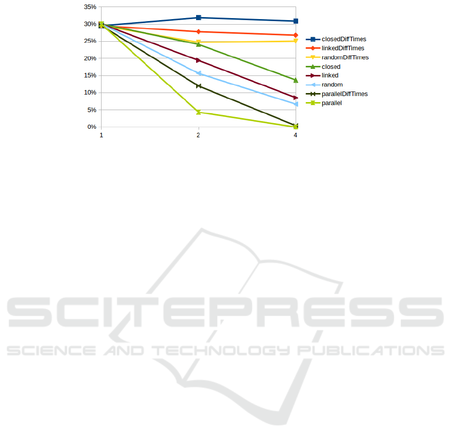
Figure 2: Average objective gaps with respect to different ﬂexibility factors 1, 2 and 4.

chine sets with machine dependent processing times

(closedDi f f Times). Here, the objective gaps even

increased slightly (though the trend turns down again

with f lex = 4). The linked machines (linked∗) and

closed machine sets (closed∗) settings were even

harder than cases with random operation to ma-

chine set assignments. Parallel machine settings

(parallel∗) are the by far easiest cases and it can be

stated that introducing new parallel machines makes it

easier to ﬁnd/prove (near-) optimal solutions. For all

different ﬂexibility types the use of machine depen-

dent processing times (∗Di f f Times) makes the prob-

lem signiﬁcantly harder for the CP Optimizer solver

to ﬁnd better solutions (or prove their optimality).

5 CONCLUSION

Referring to the three aspects identiﬁed in the intro-

duction of this paper that might have the potential to

ease the FJSSP from a practical point of view, the re-

sults of the experimental evaluation supports the as-

sumptions that:

1. Machine independent processing times, i.e. oper-

ations possess the same processing time for each

machine on which they could be processed, eases

the challenge of ﬁnding/proving (near-) optimal

solutions.

2. The architecture of a (ﬂexible job) shop, i.e. which

type of ﬂexibility is allowed/possible in a shop,

highly impacts on problem solvability. In particu-

lar, the case where ﬂexibility is based on parallel

machines each of which only supporting the same

single operation type, though still NP-hard from

a theoretical point of view, was identiﬁed to be a

quite easy type of FJSSP.

3. Increased ﬂexibility factors do not decrease the

(proven) solution quality. In contrary, in our eval-

uations the objective gap, i.e. the proven worst-

case difference between the found solution and an

optimal solution, decreased by increasing the al-

lowed ﬂexibility.

From a practical point of view the results of this

paper has several implications:

• The parallel machine FJSSP variant, that was

identiﬁed to be the easiest one, is often found also

in nowadays modern production environments.

For such application areas exact methods, in par-

ticular constraint programming (CP), should at

least be tried also in the light of large instances, as

it could be a strong alternative to heuristic meth-

ods.

• If operation processing times are machine depen-

dent but do not differ largely, it could be a good

idea to make these processing times machine in-

dependent (e.g. by using the average or the maxi-

mum) and correct the processing times in the near-

optimal solution afterwards, since machine inde-

pendent processing times lead to an easier prob-

lem variant from a practical CP point of view.

• The ﬁndings of this paper can be taken into ac-

count in order to or produce benchmark problem

instances of differing hardness.

• The often heard/read assessment that the FJSSP

is harder than the ’normal’ JSSP is not generally

true, especially when targeting at near-optimal so-

lutions.

Future work might concentrate on the following

issues:

• The results account for constraint programming

(CP). It can be assumed that the ﬁndings also

apply for other constraint based methods like

(mixed) integer programming or SAT-solving.

However, it is not clear whether heuristic methods

(e.g. evolutionary and genetic algorithms (Tep-

pan and Col, 2020; Teppan, 2018b; Teppan E.C.,

Types of Flexible Job Shop Scheduling: A Constraint Programming Experiment

521

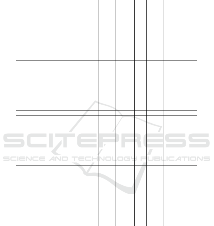
Table 1: Measured objective gaps.

# ﬂex=1 ﬂex=2 ﬂex=4 # ﬂex=1 ﬂex=2 ﬂex=4

randomDiffTimes 1 0.29 0.24 0.21 random 1 0.30 0.14 0.04

randomDiffTimes 2 0.29 0.27 0.26 random 2 0.29 0.19 0.10

randomDiffTimes 3 0.29 0.26 0.26 random 3 0.31 0.16 0.07

randomDiffTimes 4 0.29 0.22 0.26 random 4 0.29 0.13 0.05

randomDiffTimes 5 0.32 0.25 0.26 random 5 0.31 0.17 0.08

randomDiffTimes 6 0.32 0.25 0.26 random 6 0.34 0.17 0.07

randomDiffTimes 7 0.27 0.26 0.26 random 7 0.29 0.17 0.08

randomDiffTimes 8 0.29 0.24 0.23 random 8 0.30 0.14 0.06

randomDiffTimes 9 0.32 0.24 0.25 random 9 0.32 0.15 0.06

randomDiffTimes 10 0.28 0.23 0.26 random 10 0.28 0.15 0.06

avg 0.30 0.25 0.25 avg 0.30 0.16 0.07

linkedDiffTimes 1 0.29 0.28 0.27 linked 1 0.30 0.18 0.09

linkedDiffTimes 2 0.29 0.28 0.28 linked 2 0.30 0.22 0.11

linkedDiffTimes 3 0.29 0.28 0.27 linked 3 0.31 0.20 0.08

linkedDiffTimes 4 0.29 0.27 0.27 linked 4 0.29 0.17 0.07

linkedDiffTimes 5 0.31 0.30 0.28 linked 5 0.30 0.21 0.10

linkedDiffTimes 6 0.32 0.31 0.26 linked 6 0.34 0.21 0.09

linkedDiffTimes 7 0.27 0.27 0.26 linked 7 0.29 0.20 0.10

linkedDiffTimes 8 0.30 0.26 0.25 linked 8 0.30 0.17 0.07

linkedDiffTimes 9 0.32 0.26 0.27 linked 9 0.31 0.19 0.07

linkedDiffTimes 10 0.28 0.27 0.26 linked 10 0.28 0.19 0.08

avg 0.30 0.28 0.27 avg 0.30 0.19 0.09

parallelDiffTimes 1 0.29 0.13 0.00 parallel 1 0.30 0.03 0.00

parallelDiffTimes 2 0.29 0.11 0.00 parallel 2 0.29 0.06 0.00

parallelDiffTimes 3 0.29 0.12 0.04 parallel 3 0.31 0.04 0.00

parallelDiffTimes 4 0.29 0.10 0.00 parallel 4 0.29 0.02 0.00

parallelDiffTimes 5 0.32 0.14 0.00 parallel 5 0.30 0.06 0.00

parallelDiffTimes 6 0.32 0.16 0.00 parallel 6 0.34 0.06 0.00

parallelDiffTimes 7 0.27 0.11 0.00 parallel 7 0.29 0.06 0.00

parallelDiffTimes 8 0.30 0.10 0.00 parallel 8 0.30 0.03 0.00

parallelDiffTimes 9 0.31 0.10 0.00 parallel 9 0.32 0.04 0.00

parallelDiffTimes 10 0.28 0.13 0.00 parallel 10 0.28 0.03 0.00

avg 0.30 0.12 0.00 avg 0.30 0.04 0.00

closedDiffTimes 1 0.29 0.33 0.30 closed 1 0.30 0.23 0.13

closedDiffTimes 2 0.29 0.32 0.33 closed 2 0.29 0.27 0.17

closedDiffTimes 3 0.29 0.32 0.31 closed 3 0.31 0.24 0.14

closedDiffTimes 4 0.29 0.31 0.30 closed 4 0.29 0.22 0.11

closedDiffTimes 5 0.32 0.34 0.32 closed 5 0.30 0.25 0.16

closedDiffTimes 6 0.31 0.35 0.30 closed 6 0.34 0.25 0.14

closedDiffTimes 7 0.27 0.30 0.31 closed 7 0.29 0.25 0.14

closedDiffTimes 8 0.29 0.31 0.30 closed 8 0.30 0.23 0.12

closedDiffTimes 9 0.32 0.30 0.32 closed 9 0.32 0.23 0.13

closedDiffTimes 10 0.28 0.31 0.30 closed 10 0.28 0.24 0.13

avg 0.30 0.32 0.31 avg 0.30 0.24 0.14

2018), dispatching rules(Teppan, 2018a)) could

beneﬁt form this paper’s ﬁndings.

• More data sets including even larger problem in-

stances could bring further insights. In particular,

the question about whether there can be found a

phase transition, e.g. e.g. with respect to ﬂexibil-

ity factors, is imposed.

• Analysis of the makespan values should reveal

whether the decreased objective gaps measured

for settings with machine independent processing

times and with larger ﬂexibility factors are mainly

due to smaller makespans or better proven lower

bounds.

REFERENCES

Applegate, D. and Cook, W. (1991). A computational study

of the job-shop scheduling problem. ORSA Journal

on Computing, 3(2):149–156.

ICAART 2022 - 14th International Conference on Agents and Artiﬁcial Intelligence

522

Blazewicz, J., Ecker, K. H., Pesch, E., Schmidt, G., and

Weglarz, J. (2014). Handbook on Scheduling: From

Theory to Applications. Springer Publishing Com-

pany, Incorporated.

Bowman, E. H. (1959). The schedule-sequencing problem.

Operations Research, 7(5):621–624.

Brucker, P. and Jurisch, B. (1993). A new lower bound for

the job-shop scheduling problem. European Journal

of Operational Research, 64(2):156–167.

Brucker, P. and Schlie, R. (1990). Job-shop scheduling with

multi-purpose machines. Computing, 45(4):369–375.

Chaudhry, I. A. and Khan, A. (2015). A research survey:

Review of ﬂexible job shop scheduling techniques. In-

ternational Transactions in Operational Research.

Da Col, G. and Teppan, E. (2019a). Google vs IBM: A

constraint solving challenge on the job-shop schedul-

ing problem. In Bogaerts, B., Erdem, E., Fodor, P.,

Formisano, A., Ianni, G., Inclezan, D., Vidal, G., Vil-

lanueva, A., Vos, M. D., and Yang, F., editors, Proc.

35th Int. Conf. on Logic Programming (ICLP’19),

Technical Communications, volume 306 of EPTCS,

pages 259–265.

Da Col, G. and Teppan, E. (2019b). Industrial size job

shop scheduling tackled by present day cp solvers. In

Schiex, T. and de Givry, S., editors, Principles and

Practice of Constraint Programming, pages 144–160,

Cham. Springer International Publishing.

Da Col, G. and Teppan, E. (2021). Large-scale benchmarks

for the job shop scheduling problem.

Fox, M. S., Allen, B. P., and Strohm, G. (1982). Job-shop

scheduling: An investigation in constraint-directed

reasoning. In Proc. of the AAAI, pages 155–158.

Fox, M. S., Sadeh, N., and Baykan, C. (1989). Con-

strained heuristic search. In Proc. of the Eleventh In-

ternational Joint Conference on Artiﬁcial Intelligence,

pages 309–315.

Garey, M. R., Johnson, D. S., and Sethi, R. (1976).

The complexity of ﬂowshop and jobshop scheduling.

Mathematics of operations research, 1(2):117–129.

Johnson, S. (1953). Optimal Two- and Three-stage Pro-

duction Schedules with Setup Times Included. Rand

Corporation.

Keng, N. and Yun, D. Y. (1989). A planning/scheduling

methodology for the constrained resource problem. In

IJCAI, pages 998–1003.

Laborie, P. and Godard, D. (2007). Self-adapting large

neighborhood search: Application to single-mode

scheduling problems. In Proc. of MISTA-07, pages

276–284.

Laborie, P. and Rogerie, J. (2016). Temporal linear relax-

ation in ibm ilog cp optimizer. Journal of Scheduling,

19(4):391–400.

Laborie, P., Rogerie, J., Shaw, P., and Vil

ım, P. (2018).

Ibm ilog cp optimizer for scheduling. Constraints,

23(2):210–250.

Lasi, H., Fettke, P., Kemper, H.-G., Feld, T., and Hoffmann,

M. (2014). Industry 4.0. Business & information sys-

tems engineering, 6(4):239–242.

Manne, A. S. (1960). On the job-shop scheduling problem.

Operations Research, 8(2):219–223.

Muth, J. and Thompson, G. (1963). Industrial Scheduling.

International series in management. Prentice-Hall.

Rodler, P., Teppan, E., and Jannach, D. (2021). Random-

ized problem-relaxation solving for over-constrained

schedules. In Bienvenu, M., Lakemeyer, G., and Er-

dem, E., editors, Proc. of the 18th Int. Conf. on Prin-

ciples of Knowledge Representation and Reasoning

(KR’21), pages 696–701.

Sadeh, N. M. and Fox, M. S. (1996). Variable and value

ordering heuristics for the job shop scheduling con-

straint satisfaction problem. Artiﬁcial Intelligence,

86:1–41.

Sycara, K., Roth, S. F., Sadeh, N., and Fox, M. S.

(1991). Distributed constrained heuristic search.

IEEE Transactions on systems, man, and cybernetics,

21(6):1446–1461.

Taillard, E. (1993). Benchmarks for basic scheduling prob-

lems. European Journal of Operational Research,

64(2):278–285.

Teppan, E. and Col, G. (2020). Genetic Algorithms for Cre-

ating Large Job Shop Dispatching Rules, pages 121–

140.

Teppan, E. C. (2018a). Dispatching rules revisited-a

large scale job shop scheduling experiment. In 2018

IEEE Symposium Series on Computational Intelli-

gence (SSCI), pages 561–568.

Teppan, E. C. (2018b). Light weight generation of dis-

patching rules for large-scale job shop scheduling. In

Proc. of the 21st Int’l Conf on Artiﬁcial Intelligence

(ICAI’19), pages 330–333.

Teppan E.C., F. G. (2018). Heuristic constraint answer set

programming for manufacturing problems. In Hatzi-

lygeroudis, I.and Palade, V., editor, Advances in Hy-

bridization of Intelligent Methods. Smart Innovation,

Systems and Technologies, volume 85.

Types of Flexible Job Shop Scheduling: A Constraint Programming Experiment

523