Map Matching Algorithm for Large-scale Datasets

David Fiedler

1 a

, Michal

1 b

, Jan Nykl

and Pavol

Zileck

Faculty of Electrical Engineering, Artiﬁcial Intelligence Center, Czech Technical University, Prague, Czech Republic

Umotional, Prague, Czech Republic

Keywords:

Map Matching, GPS, Big Data, Graph Search.

Abstract:

GPS receivers embedded in cell phones and connected vehicles generate series of location measurements that

can be used for various analytical purposes. A common preprocessing step of this data is the so-called map

matching. The goal of map matching is to infer the trajectory that the device followed in a road network from

a potentially sparse series of noisy location measurements. Although accurate and robust map matching algo-

rithms based on probabilistic models exist, they are computationally heavy and thus impractical for processing

large datasets. In this paper, we present a scalable map matching algorithm based on Dijkstra’s shortest path

method, that is both accurate and applicable to large datasets. Our experiments on a publicly available dataset

showed that the proposed method achieves accuracy that is comparable to that of the existing map matching

methods using only a fraction of computational resources. As a result, our algorithm can be used to efﬁciently

process large datasets of noisy and potentially sparse location data that would be unexploitable using existing

techniques due to their high computational requirements.

1 INTRODUCTION

With the current spread of GPS receivers, embed-

ded into almost all cell phones and connected cars,

a huge amount of GPS data from vehicular trafﬁc is

produced. The data can be used to analyze various

properties of road network like trafﬁc density, travel

time, or speed, or to uncover trafﬁc-related behavioral

patterns. For all these applications, however, we need

to ﬁrst perform the so-called map matching, a process

of mapping the GPS records to the road network to

obtain the real path driven by the vehicle.

The map matching problems can be divided into

two categories: online map matching and ofﬂine map

matching. The online map matching is a process of

determining the path of a driving vehicle, while the

ofﬂine map matching computes the path after all GPS

measurements have been recorded. As we study the

ofﬂine map matching problem, we will use the term

“map matching” to refer to the ofﬂine map match-

ing in the remainder of this paper. While online

map matching has a broader application, including

the consumer market, ofﬂine map matching is a key

component in trafﬁc analysis. With the data about ve-

hicle movement in the road network, computed by of-

https://orcid.org/0000-0001-5374-1089

https://orcid.org/0000-0001-6450-7976

ﬂine map matching, we can analyze trafﬁc patterns

or even estimate the speed on individual road seg-

ments (Leodolter et al., 2015).

When the location data are sparse and affected

by signiﬁcant measurement errors, the map matching

problem becomes challenging because there are typ-

ically multiple routes in the road network that could

be considered as a match for the measurements. In

an urban environment, in particular, the GPS signal

is often affected by multipath propagation, which, in

conjunction with other effects, can result in a mea-

surement error larger than 20 m (Merry and Bettinger,

2019). See Figure 1a for an example of measurement

error in an urban environment. Furthermore, to keep

energy consumption low, many devices produce data

at low frequency. For example, according to Yuan

et al. (2010), 66 % of the data generated by Beijing

taxis were sampled with a frequency lower than one

sample per minute. See also Figure 1b that illustrates

the low sampling frequency problem.

To enable the processing of low-frequency high-

noise GPS data, a number of map matching algo-

rithms have been proposed (see Section 1.1). A typ-

ical map matching algorithm is based on the 2-step

scheme. First, a set of candidate projections (road

segments) on the road network is computed for each

GPS record. Then, the most probable path is chosen

500

Fiedler, D.,

Cáp, M., Nykl, J. and Žilecký, P.

Map Matching Algorithm for Large-scale Datasets.

DOI: 10.5220/0010849100003116

In Proceedings of the 14th International Conference on Agents and Artiﬁcial Intelligence (ICAART 2022) - Volume 3, pages 500-508

ISBN: 978-989-758-547-0; ISSN: 2184-433X

(a)

(b)

Figure 1: Examples of GPS sampling problems. Each red

circle represents a single GPS record. On the left, we see

an example of measurement noise of GPS records. On the

right, we can see the low sampling frequency problem.

so that for each record, there is one candidate pro-

jection in the ﬁnal path. We refer these algorithms as

global because they select the path that is globally op-

timal with respect to some model describing the map

matching problem (e.g., the minimal average distance

between a measurement and the corresponding can-

didate edge). Global map matching algorithms man-

age to match even very sparse GPS records with high

measurement errors. These algorithms are, however,

computationally heavy and thus they are impractical

for the processing of large datasets, possibly contain-

ing millions of GPS traces (see, e.g., the computa-

tional time results of Tang et al. (2016)). Other meth-

ods attempt to optimize the path locally, matching the

GPS measurements one by one. We refer to these ap-

proaches as local map matching algorithms. These

methods, however, achieve unsatisfactory accuracy,

especially on low-frequency high-noise datasets (see

the comparison in Lou et al. (2009)).

In this paper, we present a global map match-

ing algorithm that achieves accuracy comparable to

the state of the art methods using considerably less

computation time. In result, this method is suitable

for processing of large location datasets. Our con-

tribution can be summarized as follows: Firstly, we

created a map matching algorithm that is based on

graph search, a different principle than the state-of-

the-art map matching algorithms. After that, we per-

formed a theoretical analysis of the algorithm and

compared its computational complexity to two pre-

viously published map matching algorithms. Finally,

we experimentally compared the accuracy and com-

putational speed of all three algorithms on a standard

map matching dataset.

We found that the proposed algorithm has lower

computational complexity than the existing ap-

proaches, and the experimental evaluation has shown

that our approach is able to generate the underlying

route estimates with the same accuracy as existing

methods, but an order of magnitude faster.

1.1 Related Work

Early map matching algorithms, developed before the

advent of GPS-enabled smartphones, did not attempt

to recover the complete route of the vehicle, but in-

stead, they focused on ﬁnding the most likely road

segment for each measurement (White et al., 2000).

An incremental algorithm and a global optimization

approach based on Fr

echet distance were later pro-

posed by Brakatsoulas et al. (2005).

Newson and Krumm (2009) formalized map

matching using Hidden Markov Model (HMM). In

the proposed model, the authors use the network con-

nectivity and measurement error to characterize the

emission and transition probabilities of the HMM.

The HMM-based map matching proved to be robust

and accurate. The matching accuracy showed to be

almost perfect even for location measurements with

a period of 30 seconds. A similar solution using dif-

ferent formalization for global optimization was pre-

sented by Lou et al. (2009), adding temporal consis-

tency as a transition criterion. A graph search based

approach that searches for a path in the road net-

work that resembles the GPS records was presented

by Wolfson (2004). The idea is similar to the ap-

proach we propose, however, the article lacks de-

tailed description and performance evaluation against

state-of-the-art methods. Other algorithms focused on

high accuracy matching of sparse GPS data were pre-

sented by Rahmani and Koutsopoulos (2013). Kui-

jpers et al. (2016) proposed a solution that added

the k-shortest path algorithm to compute the globally

optimal path. The work by Tang et al. (2016) fol-

lows a similar direction, presenting a time-expanded

road network graph as a formalization of the problem.

In Yin et al. (2016), the authors propose a novel so-

lution that improves the accuracy by incorporating a

behavioral model in the map matching process. More-

over, they show that trajectory simpliﬁcation can be

used to speed up the map matching process. A map

matching method based on genetic algorithms was

studied by Nikoli

c and Jovi

c (2017). They compared

the accuracy of their approach with seven map match-

ing methods and showed that it outperforms all of

them with the exception of the HMM map matching

by Newson and Krumm (2009). Finally, Zhang et al.

(2021) presented a turning point based map matching

method. This method that ﬁrst splits the trajectory at

selected turning points into smaller segments and then

matches each segment separately proved to be better

both in accuracy and in matching speed than ﬁve se-

lected baseline algorithms, including works by Rah-

mani and Koutsopoulos (2013) and Kuijpers et al.

(2016).

Map Matching Algorithm for Large-scale Datasets

501

For a more comprehensive overview of existing

map matching algorithms, we refer the reader to the

existing surveys on the topic (Quddus et al., 2007;

Hashemi and Karimi, 2014; Kubicka et al., 2018;

Huang et al., 2021).

2 PROBLEM STATEMENT

We start by deﬁning the necessary terms. Road net-

work is a directed graph, in which the arcs represent

the road segments and the nodes represent either the

intersections or simply connect two following road

segments. A location measurement contains a lat-

itude, longitude, and the time of the measurement.

Location measurements are typically obtained using a

GPS receiver. A sequence of location measurements

that covers a particular period of time is called a trace.

If we connect the measurements in the trace with line

segments, we get a sequence of lines, which we call

a trace linestring. When we talk about ground truth,

we refer to a sequence of consecutive road segments

that was driven by the vehicle, while it was collect-

ing location measurements. The ground truth is used

to measure the map matching accuracy. The match is

a sequence of consecutive road segments constructed

using a map matching algorithm.

In this paper, we are interested in the map match-

ing problem, i.e., we desire to determine the ground-

truth path traversed by a vehicle in a road network

from a given trace.

3 TOWARDS MAP MATCHING

ALGORITHM FOR LARGE

DATASETS

In this section, we brieﬂy describe two existing

map matching algorithms that we used for compari-

son with our algorithm and discuss their limitations.

The Hidden Markov Model map matching algorithm

(HMM-MM) by Newson and Krumm (2009) is a

well-known example of the global map matching al-

gorithm that is both robust and accurate, outperform-

ing, in terms of accuracy, even recent map matching

methods (Nikoli

c and Jovi

c, 2017). However, it is

also computationally heavy. On the other hand, the

incremental algorithm from Brakatsoulas et al. (2005)

is an example of a local map matching algorithm that

is fast but not as accurate.

The HMM-MM is a global map matching algo-

rithm that leverages Hidden Markov Models to ﬁnd

the most probable path (sequence of road segments)

from all possible paths generated by projecting lo-

cation measurements to different edges in the road

network. The probability of each path is computed

using the emission probability (probability of visit-

ing a node) and transition probability (probability of

traveling between speciﬁc nodes). In this approach,

a measurement noise model is used to determine the

emission probability, while the transition probability

is inferred from the difference between Euclidean and

road network distance.

The incremental algorithm by Brakatsoulas et al.

(2005) ﬁrst ﬁnds the initial edge by choosing it from a

set of candidate edges that lie within a given threshold

distance from the ﬁrst location measurement. Then,

in each step, it tries to match the next measurement to

one of the road segments that are connected to the pre-

viously matched edge. The algorithm can also utilize

a look-ahead strategy: it tries to match a few location

measurements ahead and propagates the score back

in an attempt to avoid myopic choices that cannot be

reversed later on in the process.

4 THE GRAPH SEARCH BASED

MAP MATCHING

In this section, we present the proposed map match-

ing algorithm: the Graph Search Based Map Match-

ing (GSMM). In contrast to simple geometric algo-

rithms (White et al., 2000), the incremental algorithm,

or the HMM-MM (both described in the previous sec-

tion), the proposed algorithm does not iterate over the

location measurements in the trace. It searches the

road network graph using a standard graph search al-

gorithm, but instead of searching for the shortest path,

it searches for the path most similar to the location

measurements. In other words, the cost of each arc in

the search graph encodes the likelihood of the edge

being part of the ground truth path given the loca-

tion measurements. We use Dijkstra’s shortest path

algorithm for graph search as it is simple, well stud-

ied, and does not require any heuristic. While Dijk-

stra’s algorithm is outperformed by A* in most appli-

cations, it is hard to imagine to use it in our case, as

there is no straightforward heuristic with the required

properties (consistency and admissibility). However,

a bidirectional variant of our algorithm can be exam-

ined in the future.

The pseudocode of the proposed algorithm is in

Algorithm 1. We start by initializing the priority

queue Q and by adding the start node n

to it with

priority 0. Then, we continue by a standard Dijkstra-

style loop, during which we add every neighbor n of

current node n

into the queue. The algorithm ends

ICAART 2022 - 14th International Conference on Agents and Artiﬁcial Intelligence

502

Algorithm 1: GSMM algorithm core.

add n

to Q with priority 0;

while Q is not empty do

← head of Q;

if n

not closed then

set n

as closed;

if n

= n

then

backtrack ;

for n ∈ neighbors of n

if n not closed then

c ← compute cost(n);

add n to Q with priority c;

when the destination node n

is reached, or when the

queue is empty (which cannot happen unless the road

network is not a strongly connected graph). The criti-

cal part of the algorithm is the initialization discussed

in Section 4.1, and the node cost computation ex-

plained in Section 4.2.

4.1 Start and end Point Determination

Determination of the start and the destination node

is the essential part of the algorithm. Unlike many

other algorithms, our solution can recover from a bad

choice of the initial node, but a mistake in initializa-

tion can still affect the accuracy. The initial edge e

chosen from the set of edges E as

= argmin

e∈E

,e| + |n

,t|. (1)

where r

is the ﬁrst location measurement, n

is the

end node of the edge e and t is the trace linestring

built by sequentially connecting all location measure-

ments. Figure 2 visualizes the cost computation of a

candidate initial edge. For performance reasons, we

add to the set E only the edges that are closer to r

than a given threshold. In our experiments, we use

the threshold of 100 m. When the initial edge is com-

puted, the start node of the edge is chosen as an initial

point n

An analogous process is performed when deter-

mining the destination point. Instead of the ﬁrst mea-

surement, we use the last measurement, and instead of

the end point of the candidate edge, we use the start

point.

4.2 Computing Edge Costs

For each neighbor node n, the total cost is computed

as a sum of the cost of the current node and the cost of

the neighbor. The cost of each neighbor is computed

Figure 2: Initialization example. Green points represent the

location measurements, gray lines are the roads, currently

evaluated edge is highlighted in black. The initial edge is

chosen such that it minimizes the sum of the distance be-

tween the ﬁrst measurement and the edge (blue dashed line),

and the distance between edge endpoint and the trace (red

dashed line).

c = (c

+ c

/α + c

, (2)

where the cost c

= |n,t| is the distance of the neigh-

bor node from the trace, and cost c

= |p

mid

,t| is com-

puted as a distance between the middle point p

mid

the edge and the trace. These costs have to be multi-

plied by the length of the edge l

to normalize them to

the edge length. The constant α controls the contribu-

tion of cost c

that represents the difference between

the length of the edge and the distance between the

current and the neighbor node projections on the trace

linestring:

= |l

− l

trace

|, (3)

where

trace

= ||p

, p

n,t

trace

. (4)

The purpose of these costs can be explained in

the following series of examples. In Figure 3a, the

computation of cost c

is illustrated. An important as-

pect that can be seen in this ﬁgure is that the cost for

nodes n

and n

is not the Euclidean distance to the

trace. The reason for this is that the algorithm always

projects the nodes on the trace chronologically and

consequently a neighbor node n cannot be projected

before the current node n

, that was already projected

to the trace in the previous step.

The cost c

is computed analogously to the cost

, the difference being that we project the middle

point of the edge, p

mid

, instead of the neighbor node.

The purpose of the cost c

is illustrated in Figure 3b,

where we can see a situation in which relying on

the cost c

would not sufﬁce to determine the correct

edge.

We could add more such control points as costs,

but our experiments suggest that this is not effective

as there were always cases for which the number of

control points was insufﬁcient. Instead, we created

another cost c

that is designed to cover the remain-

ing cases by comparing the length of the edge and the

length along the trace between the projection of the

Map Matching Algorithm for Large-scale Datasets

503

(a)

(b)

(c)

Figure 3: Illustration of computation of cost c

(a), c

(b), and c

(c). The costs are represented by blue dashed lines, the green

points are the location measurements, the white circle is the current node, and the black circles and lines represent the road

network nodes and edges, respectively. Note that in Figure a), the cost for nodes n

and n

is not the Euclidean distance to

the trace because the neighbors have to be projected after the current point. On the second picture, we can see that the middle

points (grey circles) can determine the correct edges even if the incorrect neighbor point has the lowest cost c

(gray dashed

line). Finally the cost c

is computed for the neighbor node n

as the absolute value of the difference between the edge length

(blue dashed line) and the length along the trace (red dotted line). We can see that both cost c

and cost c

(gray dashed lines)

would mistakenly chose n

as the match.

Figure 4: The example of ambiguous projection of the

node. We can see the nearest projection and one alterna-

tive projection on the picture, depicted as the blue dashed

line.

current node n

on the trace (which was ﬁxed in the

previous step of the algorithm) and the projection of

the neighbor node n. We can see the example where

this metric is essential to correctly match the trace in

Figure 3c.

Sometimes, the vehicle completely changes its di-

rection during a single trip. In this case, the projec-

tion of a speciﬁc edge on the trace linestring can be

ambiguous, i.e., multiple points in the trace can have

a similar distance to the edge, despite being very far

from each other along the trace (see Figure 4). We

solve such cases by providing alternative projections

that are in the same and in the opposite direction of the

nearest projection within a distance of 100 m. Then,

we compute the total cost c for each candidate projec-

tion and choose the projection with the lowest cost.

After choosing the best projection for the candi-

date neighbor node, we apply another cost c

to the

cost sum, resulting in the equation

= c + c

, (5)

where c is the neighbor cost deﬁned above and c

computed as

= −β||p

, p

n,t

trace

. (6)

In the above equation, ||p

, p

n,t

trace

is the distance

along the linestring between current and neighbor

node projection and β is the forward heuristic coef-

ﬁcient. The weight c

is a heuristic that guides the

search and speeds up the computation, as the edges

that lead forward along the trace have a lower cost.

By assigning higher values for β, we can speed up the

computation signiﬁcantly, but higher values can also

lead to less accurate results.

5 DISCUSSION

In this section, we discuss the computational com-

plexity, performance, advantages, and limitations of

the three compared algorithms.

5.1 Complexity

The worst-case asymptotic complexity of the GSMM

algorithm is identical to Dijkstra’s algorithm, O(|E|+

|N| · log |N|), where |E| is the number of road seg-

ments and |N| is the number of road network nodes.

The computational complexity of the HMM-based

method is dominated by the Viterbi’s algorithm,

O(|R|·|E|

), where |R| is the number of location mea-

surements in the trace. The complexity of the incre-

mental algorithm is O(|R|). In practice, however, such

worst-case complexities are never reached, partly due

to the structure of the input and partly due to the per-

formance optimization tricks that would be applied in

the case of practical deployment.

In HMM map matching, the complexity is reduced

by considering only nodes within a ﬁxed radius from

the location measurement as candidates – this drasti-

cally reduces the number of edges |E| considered by

Viterbi’s algorithm. In GSMM, the worst case com-

plexity is also virtually never reached, because due to

ICAART 2022 - 14th International Conference on Agents and Artiﬁcial Intelligence

504

the design of the cost function, the search is focused

on the vicinity of the trace.

Finally, real-world traces typically contain only

tens to hundreds of location measurements. In re-

sult, the time spent on computations that depends

on the dataset size |R| can be easily dominated

by constant-time computations. This can be easily

demonstrated in the incremental algorithm, where the

worst-case time complexity is exponential with re-

spect to the lookahead depth d

. For d

= 4, as used by

Brakatsoulas et al. (2005) and a conservative average

branching factor b = 4, the complexity of evaluation

of each step, which can be expressed as O(b

), easily

dominates the measurement count.

An important difference between the GSMM and

other map matching algorithms regarding the com-

plexity is that the complexity of the GSMM is not

directly related to the number of location measure-

ments. In the case of other algorithms, both global

and local, the number of algorithm steps is linearly

dependent on the number of measurements. In re-

sult, these algorithms are not suitable for dense traces,

sometimes even removing a signiﬁcant number of

measurements from traces is proposed to speed up the

algorithm (Yin et al., 2016).

5.2 Performance, Advantages, and

Limitations of Our Solution

The main shortcoming of the incremental algorithm

is that it can choose wrong edges for the match be-

cause the lookahead has only a constant depth and the

edge cannot be changed once chosen for a projection

of a location measurement. In contrast, the HMM-

MM and the GSMM search for a match with a glob-

ally optimal score. Yet, the probabilities in HMM-

MM and edge costs in GSMM are nothing more than

a model that uses the sensor data and network topol-

ogy. In addition, the optimality of the HMM map

matching is affected by the fact that it only searches

for measurement projection candidates below a given

distance threshold.

As it is clear from the Section 4.2 describing the

computation of the weights, GSMM tries to ﬁnd the

path in the road network that is most similar to the

vehicle trace. This produces correct results most of

the time, but in sparse traces, sometimes, the path that

is more distant from the trace could be correct as it

is demonstrated in Figure 5. One of the techniques

that can be used to match these scenarios correctly

is described by Osogami and Raymond (2013) and

also by Yin et al. (2016). This technique could be

incorporated in the GSMM in the form of an addi-

tional cost. Other aspects of human behavior, such

Figure 5: An example case of a problematic matching re-

lated to sparse traces. The green path is closer to the trace,

but the ground-truth path is the blue path.

as temporal consistency, can be modeled as well, by

simply adding the respective costs. Another advan-

tage of the GSMM is that the edge costs are easy to

compute. In contrast, in the HMM-MM, the short-

est path needs to be computed to evaluate each transi-

tional probability. The need for such frequent shortest

path computation is a signiﬁcant shortcoming. In fact,

we observed that in our implementation, the shortest-

path computations account for 98% of the runtime.

Moreover, due to the ability of the GSMM to do fast

matching, as demonstrated in Section 6.1, we believe

that the GSMM can be used for online map matching

too, simply by performing the map matching on all

location measurements available so far.

The only limitation of our method are cycles in

traces. Because the GSMM is based on Dijkstra al-

gorithm, it is not able to correctly match traces con-

taining cycles. In practice, however, we simply break

self-intersecting traces in parts and match each part

separately.

6 BENCHMARK

We experimentally compared the GSMM, the HMM-

MM, and the incremental approach using an exist-

ing benchmark dataset

containing traces together

with road networks and ground truths (Kubicka et al.,

2018). The dataset does not contain “clean” traces,

but instead, the traces contain artifacts like gaps or

hives (a large number of measurements in a certain

area) that are challenging for map matching algo-

rithms. The traces in the dataset have the measure-

ment period of one second, longer periods were cre-

ated by our benchmark by subsampling the original

trace. Eleven period lengths between 1 second to 5

minutes length were tested. The period of 24 seconds

represents the average measurement period measured

on a real dataset of almost 10 thousand taxi trips in

Prague collected by a ride-hailing application Liftago.

The complete histogram of the delays between points

in the Prague dataset is in Figure 6. Because our al-

https://zenodo.org/record/57731

Map Matching Algorithm for Large-scale Datasets

505

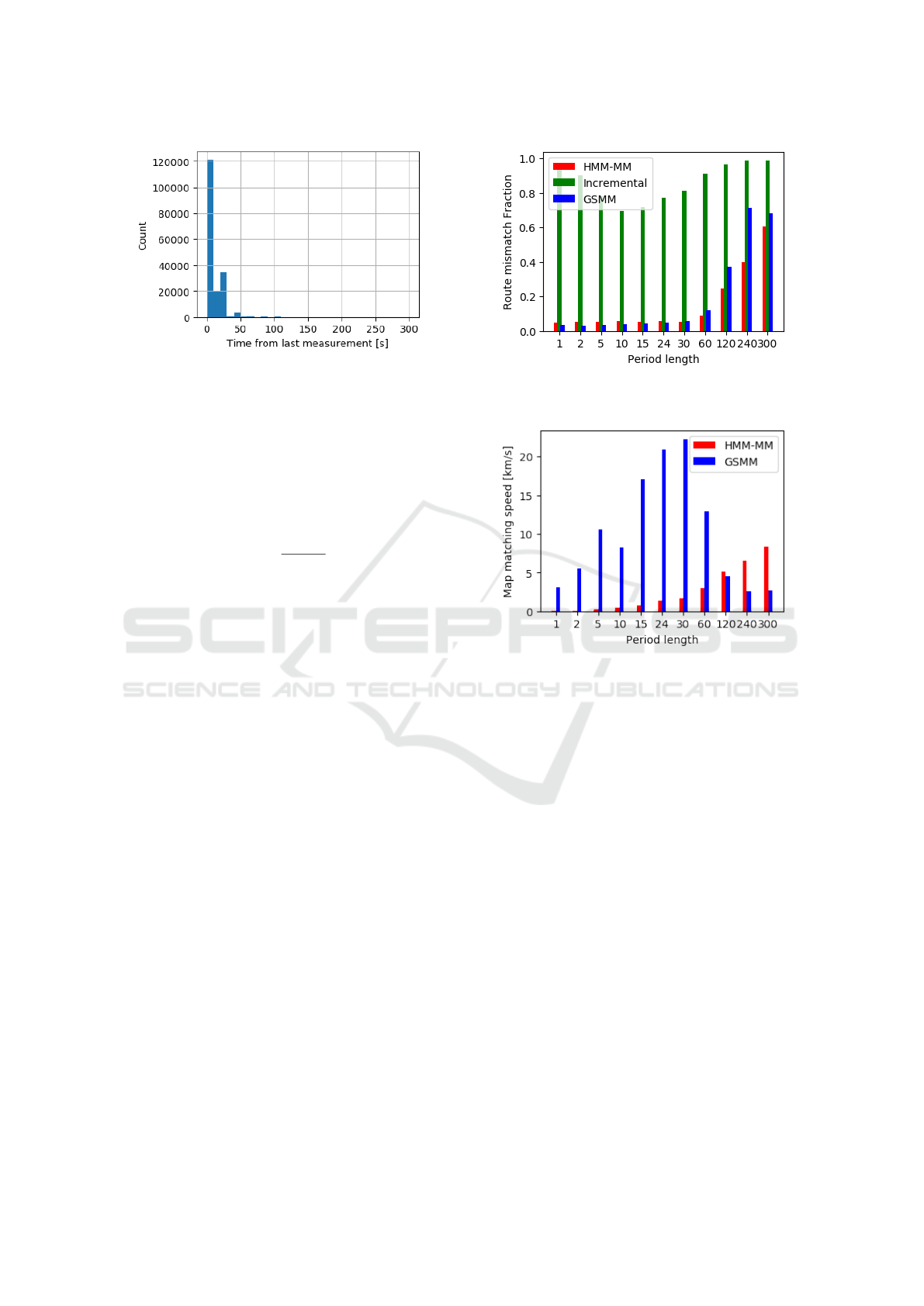
Figure 6: Histogram of delay between the traces from

Prague taxi trace dataset.

gorithm cannot handle traces containing cycles, only

a subset of traces without cycles was used for evalua-

tion.

To measure the map matching accuracy, we used a

metric called Route Mismatch Fraction (RMF) intro-

duced by Newson and Krumm (2009). The RMF is

computed as

RMF =

+ l

−

, (7)

where l

is the ground truth length, l

is the length of

the segments in the match that are not in the ground

truth (false positive length), and l

−

is the length of the

segments in the ground truth not present in the match

(false negative length).

All algorithms and the benchmark were imple-

mented in Python and ran on a desktop PC with In-

tel Core i5 4950S CPU and 24 GB of memory. The

HMM-MM algorithm was conﬁgured with parame-

ters σ = 50 and β = 2, edges in the radius of 15 meters

were considered as projection candidates. For the in-

cremental algorithm, the parameters were conﬁgured

as follows: µ

= 10,n

= 1,a = 0.17,mu

= 10,n

7. The look-ahead depth was set to 4, the start area ra-

dius was set to 100 m, and max allowed skipped edges

was set to 10. In the GSMM, the start area radius was

set to 100 m and the forward heuristic cost weight β

was set to 3.

6.1 Results

The comparison of the accuracy of the tested algo-

rithms is in Figure 7. As we can see, the accuracy of

the incremental algorithm is very low. Thus, we de-

cided to remove the incremental algorithm from other

comparisons, as it is clearly not able to produce rea-

sonable matches for the benchmark dataset. The ac-

curacy of the GSMM is comparable to HMM-MM up

to the period of 30 s, which is more than the aver-

age measurement period measured on the real-world

Figure 7: Comparison of the accuracy of the three evaluated

algorithms on traces with different sampling frequencies.

Figure 8: Comparison of speed of the GSMM and the

HMM-MM on traces with different sampling frequencies.

dataset (Section 6). For periods above 30 s, the ac-

curacy of both algorithms starts to degrade, with the

GSMM declining more rapidly. Concerning the speed

(Figure 8), the GSMM is faster than the HMM-MM

up to the period of two minutes, under one minute pe-

riod, our algorithm is more than ten times faster.

The ﬁrst thing to explain is the failure of the in-

cremental algorithm to provide reasonable matches.

We investigated that the algorithm fails on the net-

work areas with very short road segments, where a

large number of road segments with similar costs can

be assigned to the location measurement. We believe

that authors of the algorithm measured the accuracy

on a simpliﬁed road network, where these problems

are rare and therefore obtained better results.

For traces with a sampling period of up to one

minute, the GSMM is signiﬁcantly, often an order

of magnitude, faster. For longer periods, the HMM-

MM dominates in speed. This is not a surprise, as

for HMM-MM, the complexity depends on the num-

ber of records (see Section 5.1). The speed should,

therefore, increase with a decreasing sampling fre-

quency, which was conﬁrmed by the results. Addi-

ICAART 2022 - 14th International Conference on Agents and Artiﬁcial Intelligence

506

tionally, in global map matching algorithms, the run-

time is strongly affected by the number of projection

candidates. In the HMM-MM, the number of can-

didates is limited by the ﬁxed radius (Newson and

Krumm, 2009), which was set to 15 m in the bench-

mark. However, in the case of a more noisy dataset,

this limit would have to be increased to obtain accu-

rate results, decreasing the speed as a result.

7 CONCLUSION

The cell phones and connected cars produce large

amounts of location data that can be used for various

analytical purposes. E.g., this data can be exploited

to estimate free-ﬂow speeds or trafﬁc densities in a

road network. A common preprocessing step is map

matching, where we desire to infer the path of the ve-

hicle through the road network from sparse and noisy

location measurements.

Many map matching algorithms have been pro-

posed that excel in accuracy or robustness with re-

spect to sparse and noisy GPS traces. Yet, with the

increasing size and availability of location measure-

ment datasets, the processing speed of map matching

algorithm becomes important.

We proposed Graph Search based map match-

ing (GSMM), a map matching algorithm based on

Dijkstra’s algorithm for the shortest path that is fo-

cused on reducing the computational complexity. We

compared the performance of the GSMM together

with a state-of-the-art global map matching algorithm

(HMM-MM) and one incremental map matching al-

gorithm on a standard, publicly available dataset.

The results show that the accuracy of the incre-

mental algorithm is unsatisfactory. Concerning the

HMM map matching, our algorithm is up to 10 x

faster and it achieves higher accuracy than the HMM

algorithm for records with a sampling period shorter

than one minute. For lower sampling frequencies, the

HMM-MM performs better, however, the real data

from a taxi company shows that such low sampling

frequencies are rare.

In the future, we would like to extend this method

with other costs that incorporate behavioral aspects.

Moreover, we plan to utilize the matched data to de-

liver a road speed model.

ACKNOWLEDGEMENT

The authors acknowledge the support of the OP

VVV MEYS funded project CZ.02.1.01/0.0/0.0/

16 019/0000765 ”Research Center for Informatics”.

REFERENCES

Brakatsoulas, S., Pfoser, D., Salas, R., and Wenk, C. (2005).

On Map-matching Vehicle Tracking Data. In Pro-

ceedings of the 31st International Conference on Very

Large Data Bases, VLDB ’05, pages 853–864, Trond-

heim, Norway. VLDB Endowment.

Hashemi, M. and Karimi, H. A. (2014). A critical review

of real-time map-matching algorithms: Current issues

and future directions. Computers, Environment and

Urban Systems, 48:153–165.

Huang, Z., Qiao, S., Han, N., Yuan, C.-a., Song, X., and

Xiao, Y. (2021). Survey on vehicle map matching

techniques. CAAI Transactions on Intelligence Tech-

nology, 6(1):55–71.

Kubicka, M., Cela, A., Mounier, H., and Niculescu, S. I.

(2018). Comparative Study and Application-Oriented

Classiﬁcation of Vehicular Map-Matching Methods.

IEEE Intelligent Transportation Systems Magazine,

10(2):150–166.

Kuijpers, B., Moelans, B., Othman, W., and Vaisman,

A. (2016). Uncertainty-Based Map Matching: The

Space-Time Prism and k-Shortest Path Algorithm.

ISPRS International Journal of Geo-Information,

5(11):204.

Leodolter, M., Koller, H., and Straub, M. (2015). Estimat-

ing travel times from static map attributes. In 2015

International Conference on Models and Technolo-

gies for Intelligent Transportation Systems (MT-ITS),

pages 121–126.

Lou, Y., Zhang, C., Zheng, Y., Xie, X., Wang, W., and

Huang, Y. (2009). Map-matching for Low-sampling-

rate GPS Trajectories. In Proceedings of the 17th

ACM SIGSPATIAL International Conference on Ad-

vances in Geographic Information Systems, GIS ’09,

pages 352–361, New York, NY, USA. ACM.

Merry, K. and Bettinger, P. (2019). Smartphone GPS ac-

curacy study in an urban environment. PLOS ONE,

14(7):e0219890.

Newson, P. and Krumm, J. (2009). Hidden Markov Map

Matching Through Noise and Sparseness. In Proceed-

ings of the 17th ACM SIGSPATIAL International Con-

ference on Advances in Geographic Information Sys-

tems, GIS ’09, pages 336–343, New York, NY, USA.

ACM.

Nikoli

c, M. and Jovi

c, J. (2017). Implementation of generic

algorithm in map-matching model. Expert Systems

with Applications, 72:283–292.

Osogami, T. and Raymond, R. (2013). Map Matching with

Inverse Reinforcement Learning. In Proceedings of

the Twenty-Third International Joint Conference on

Artiﬁcial Intelligence, IJCAI ’13, pages 2547–2553,

Beijing, China. AAAI Press.

Quddus, M. A., Ochieng, W. Y., and Noland, R. B. (2007).

Current map-matching algorithms for transport appli-

cations: State-of-the art and future research directions.

Transportation Research Part C: Emerging Technolo-

gies, 15(5):312–328.

Rahmani, M. and Koutsopoulos, H. N. (2013). Path infer-

ence from sparse ﬂoating car data for urban networks.

Map Matching Algorithm for Large-scale Datasets

507

Transportation Research Part C: Emerging Technolo-

gies, 30:41–54.

Tang, J., Song, Y., Miller, H. J., and Zhou, X. (2016). Esti-

mating the most likely space–time paths, dwell times

and path uncertainties from vehicle trajectory data:

A time geographic method. Transportation Research

Part C: Emerging Technologies, 66:176–194.

White, C. E., Bernstein, D., and Kornhauser, A. L. (2000).

Some map matching algorithms for personal navi-

gation assistants. Transportation Research Part C:

Emerging Technologies, 8(1):91–108.

Wolfson, a. O. (2004). A weight-based map matching

method in moving objects databases. In Proceed-

ings. 16th International Conference on Scientiﬁc and

Statistical Database Management, 2004., pages 437–

438.

Yin, Y., Shah, R. R., and Zimmermann, R. (2016). A Gen-

eral Feature-based Map Matching Framework with

Trajectory Simpliﬁcation. In Proceedings of the

7th ACM SIGSPATIAL International Workshop on

GeoStreaming, IWGS ’16, pages 7:1–7:10, New York,

NY, USA. ACM.

Yuan, J., Zheng, Y., Zhang, C., Xie, X., and Sun, G.-Z.

(2010). An Interactive-Voting Based Map Matching

Algorithm. In 2010 Eleventh International Confer-

ence on Mobile Data Management, pages 43–52.

Zhang, D., Dong, Y., and Guo, Z. (2021). A turning point-

based ofﬂine map matching algorithm for urban road

networks. Information Sciences, 565:32–45.

ICAART 2022 - 14th International Conference on Agents and Artiﬁcial Intelligence

508