Queueing Model of Circular Demand Responsive Transportation

System: Theoretical Solution and Heuristic Solution

Ayane Nakamura

, Tuan Phung-Duc

1 a

and Hiroyasu Ando

2,3 b

Graduate School of Science and Technology, University of Tsukuba, Tsukuba, Ibaraki 305-8577, Japan

Faculty of Engineering, Information and Systems, University of Tsukuba, Tsukuba, Ibaraki 305-8577, Japan

Advanced Institute for Materials Research, Tohoku University, Sendai, Miyagi 980-8577, Japan

Keywords:

Queueing Model, Transportation, Ride-sharing, Heuristic Solution.

Abstract:

Sharing mobilities, such as car-sharing and ride-sharing, have been widely spreading recently. In this paper, we

consider Car/Ride-Share (CRS) system, which is one of the demand responsive transportations. We consider

the scenario where CRS is introduced on the circular bus route. We propose its theoretical and heuristic

solutions using queueing theory. We validate the heuristic analysis by comparing with the theoretical result

through some numerical examples.

1 INTRODUCTION

Sharing mobilities, such as car-sharing and ride-

sharing have been widely spreading recently. Car-

sharing is a system such as car-rental for short period

time and ride-sharing is a system where people ride

cars to their destinations together, e.g., Uber. In this

paper, we study Car/Ride-share (CRS) system (Ando

et al., 2019), where people carry out car-sharing and

ride-sharing simultaneously. We analyzed a queue-

ing model where CRS is introduced between two

points (Nakamura et al., 2020a). As an extension,

we model and analyze the scenario of the introduc-

tion of CRS on a circular bus route. As we will de-

scribe later, the theoretical analysis of the multiple

points model requires a huge amount of computaiton

and memory capacity when conducting numerical ex-

periments. Therefore, we propose a heuristic solution

of the model to facilitate the numerical experiments.

We compare these two solutions, the theoretical and

the heuristic solutions, and discuss the validity of the

heuristic solution.

There are various studies about sharing mobili-

ties. Speciﬁcally, , various studies using optimization

method were conducted, e.g., (Agatz et al., 2012),

(Correia and Antunes, 2012). However, almost all of

these studies ignore the uncertainty of customer be-

haviors. In other words, these studies assume that

https://orcid.org/0000-0002-5002-4946

https://orcid.org/0000-0003-1102-2291

all customer behavior is perfectly understood. In re-

ality, customer behavior has ﬂuctuation. Naturally

that sometimes there are many customers and some-

times there are few because of external factors such

as other transportations, the road congestion, weather,

and so on. A closely related study (Enzi et al., 2021),

which deals with the scheduling problem of multi-

modal car- and ride- sharing problem, also ignores the

uncertainty of customers.

As research considering the randomness of cus-

tomers, Daganzo et al. (Daganzo and Ouyang, 2019)

discussed a simple stochastic model of demand-

responsive transportations that include ride-sharing.

However, they did not consider the coexistence of

multiple transportations, e.g., buses and ride-sharing.

It is crucial to discuss the coexistence of various mo-

bilities and evaluate the impact on each other from a

practical point of view. Research of queueing mod-

els for transportation services (e.g., (Tao and Pender,

2020)) also did not consider the coexistence of vari-

ous types of mobilities.

Based on the above, the novelties of this paper can

be summarized as follows:

• Modeling transportation systems considering the

uncertainty of customers.

• Modeling the coexistence of multiple transporta-

tions, i.e., Car/Ride-Share.

• Presenting both theoretical and heuristic solutions

for this new model.

Nakamura, A., Phung-Duc, T. and Ando, H.

Queueing Model of Circular Demand Responsive Transportation System: Theoretical Solution and Heuristic Solution.

DOI: 10.5220/0010845300003117

In Proceedings of the 11th International Conference on Operations Research and Enterprise Systems (ICORES 2022), pages 193-199

ISBN: 978-989-758-548-7; ISSN: 2184-4372

193

The rest of the paper is organized as follows. In Sec-

tion 2, we describe the model based on queueing the-

ory. Sections 3 and 4 present theoretical and heuristic

solutions. Section 5 shows some numerical results.

The ﬁnal section of the paper, Section 6, presents a

discussion and concluding remarks.

2 MODELING

This section presents the modeling of our scenario for

CRS system on a circular bus route.

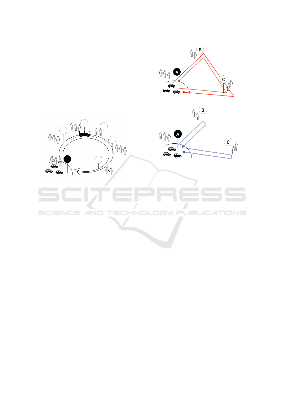
Figure 1: Schematic illustration of the modelling.

We consider a circular bus route as Figure 1. We

assume that there is a car parking lot for CRS at one

of the bus stops (the bus stop is painted black in Fig-

ure 1). In the CRS system, car providers provide their

private cars for ﬁnancial incentives (Nakamura et al.,

2020a). This mechanism refers to the concept of peer-

to-peer car-sharing, where people lend their private

cars. We discussed the beneﬁcial price mechanism

for the car providers between two points (Nakamura

et al., 2020b). In this paper, we focus on the model

extended to capture the travel among multiple points.

Therefore, as the ﬁrst step in the research of the mul-

tiple points model, we do not consider detailed ﬁ-

nancial discussion for system participants such as car

providers in this research. Of course, it is vital to dis-

cuss its ﬁnancial perspective to aim for practical use.

On the circular bus route, buses are operated based

on a ﬁxed schedule. This model assumes that a bus ar-

rives according to the interval that follows an Erlang

distribution with rate r and shape q (this means the

sum of q exponentially distributed random variables

of parameter r). Erlang distribution can approximate

a constant value, i.e., this assumption is suitable for

modeling the ﬁxed bus schedule. Erlang distribution

can be constructed by a convolution of exponential

distributions. Therefore, this approximation makes

the model easier to be analyzed as a Markov chain.

Now, we deﬁne the concept of “class” of the cus-

tomers. A class means the combination of the bus

Figure 2: The routes of CRS when N = 3.

stop where the customers ﬁrst arrive, and the bus stop

that is the ﬁnal destination of the customer. For ex-

ample, class-AB is for the customers who wait for the

bus coming at the bus stop A, and wants to visit bus

stop B ﬁnally. Besides, we assume that customers of a

class arrives at a bus stop according to a Poisson pro-

cess with a distinct parameter for that class, e.g., the

customers of class- AB arrive according to the Pois-

son Process of rate λ

. We also assume the cus-

tomers ride on the buses within the designated number

of people for each class, e.g., the customers of class-

AB get on a bus up to X

(which follows an arbitrary

distribution) customers.

We consider the scenario of the introduction of

CRS on this circular bus route aiming to reduce con-

gestion for the customers. The speciﬁc description of

the CRS system is as follows:

• Car providers provide their private cars for the

parking lot to gain ﬁnancial incentives, i.e., car-

sharing.

• Customers can ride the cars with other customers

who have the same direction, i.e., ride-sharing.

From these explanations, we can understand that CRS

is a hybrid system of car-sharing and ride-sharing.

What is very different from buses is that CRS is

demand-responsive type transportation, i.e., CRS is a

system where a car does not depart unless more than a

certain number of people want to use it. Besides, cars

of CRS should be returned to their original position

(i.e., the parking lot) after the CRS travel. Therefore,

ICORES 2022 - 11th International Conference on Operations Research and Enterprise Systems

194

it is necessary to match the trips that enable the car to

ﬁnally return to the parking lot. This constraint seems

to be troublesome at ﬁrst glance. However, it would

reduce the cost of relocating the cars by the operator

in traditional car-sharing systems. In our scenario, we

assume that the operator of CRS (that can be an op-

erating company dedicated to CRS, and the bus com-

pany itself) controls the occurrences of CRS under a

particular policy. As a simple policy, we assume the

following:

• The minimum and the maximum capacities of the

car are m and n customers, respectively.

• We ignore the lack of cars and whether customers

have a driver license or not to simplify the model.

• We deﬁne the “route” as the course of CRS that

starts and ends with the bus stop where there is

the parking lot.

• For example, we assume that there are three bus

stops (A, B, and C) on circular, and there is the

parking lot of CRS at the bus stop-A (see Figure

2). Note that we call a bus stop “node” to the sim-

pliﬁed expression and deﬁne N as the number of

nodes afterward. The possibilities of the routes

are as follows:

– A → B → C → A

– A → C → B → A

– A → B → A

– A → C → A

• Supplementary deﬁnitions of the route are as fol-

lows: it is impossible to visit the same node more

than once except for the bus stop where there is

the parking lot, e.g., A → B → C → B → A is im-

possible in the setting of Figure 2.

• If there are m or more customers of all classes

that composes a route, CRS of its route occurs

according to the interval which follows the expo-

nential distribution of parameters given for each

route. For example, this is because it takes time

for matching of customers by the operator of CRS

through the control system, e.g., web application

on smartphone. At the moment of the comple-

tion of the matching, maximum number of cus-

tomers not exceeding n (the maximum capacity

of the car) ride on the car and start to drive. Note

that we do not consider who drives the car in this

paper.

• Considering the example in Figure 2, CRS of

route A → B → C → A occurs according to the in-

terval which follows the exponential distribution

with rate σ

ABC

, on the condition that the num-

ber of all class-AB, class-BC and class-CA is m

or more people. In other words, the customers of

class-AB start driving from node-A to node-B, and

they get off the car at the node-B. The customers

of class-BC take over the car at node-B and go to

node-C. After that, the customers of class-CA start

to drive to node-A (the parking lot). By this series

of ﬂow, the car is returned to its original position.

The same is true for other routes.

• Supplementary explanation about the car

takeover; customers of different classes from

same node would not ride the same car, e.g.,

class-AB and class-AC can not be in same car.

In the next section, we show the theoretical solution

of the scenario using queueing theory.

3 THEORETICAL ANALYSIS

In this section, we show the theoretical analysis of

the model. For simplicity, we describe the example

analysis where the number of nodes (N) is 3, as in the

previous section. Then, we summarize the parameters

and the variables used in the analysis in Table 1.

Table 1: Parameters used in the analysis.

Parameters Deﬁnitions

N The number of nodes.

The arrival rate for the customers

of class-G.

m The minimum capacity of CRS cars.

n The maximum capacity of CRS cars.

The random variable of

the number of customers

who get into a bus in class-G.

Parameters of Erlang distribution of

the interval of buses at node-G.

The occurrence rate of CRS

for route-G.

The capacity for the customers

in node-G.

First of all, we deﬁne some sets as follows: S

{0,1,2,...,K

− 1, K

}, S

= {0,1,2,...,K

−

1,K

}, S

= {0, 1, 2, . . . , K

− 1,K

}, S

{0,1,2,...,K

− 1,K

}, S

= {0,1,2,...,K

−

1,K

}, S

= {0, 1, 2, . . . , K

− 1,K

}, R

{0,1,2,...,r

− 2,r

− 1}, R

= {0,1,2,...,r

−

2,r

− 1}, R

= {0,1,2,...,r

− 2,r

− 1}, and Z =

× S

× R

Let S

(t), S

(t) and

(t) denote the number of the waiting cus-

tomers for each class at time t, respectively, and

(t), R

(t) and R

(t) denote the progress of

Queueing Model of Circular Demand Responsive Transportation System: Theoretical Solution and Heuristic Solution

195

the Erlang distributions for buses at each node

at time t, respectively. It is easy to ﬁnd that

{(S

(t),S

(t),R

(t),

(t),R

(t));t ≥ 0} forms a Markov chain in the

state space Z.

Because the Markov chain is ﬁnite and irre-

ducible, we deﬁne the steady state probabilities as fol-

lows:

( j

, j

)

= lim

t→∞

P(S

(t) = j

(t) = k

where i

∈ S

, i

∈ S

, i

∈ S

, i

∈ S

, i

∈

, i

∈ S

, k

∈ R

, k

∈ R

, k

∈ R

Sorting the all the states in Z in the lexi-

cographic order, the inﬁnitesimal generator Q

Q =

(size: ((K

+ 1)(K

1)(K

+ 1)r

)) of our Markov chain is given as

follows:

Q =







0 1 2 ...

0 Q

1 Q

2 Q

Y Q

y,e

y,y







where

Y = ((K

+ 1)(K

1)(K

+ 1)(K

+ 1)r

) − 1,

y = (K

− 1,r

−

1,r

− 1), e

= (0,0,0,0,0,0,0,0,0), e

(0,0,0,0,0,0,0,0,1), e

= (0,0,0,0,0,0,0,0,2).

Moreover, we also deﬁne the elements of

Q as follows (for subscripts, we write only

where there is a main change in transition):

(...,k

),(...,k

+1,k

)

= q

, 0 5 k

5 r

− 2,

(...,k

),(...,k

+1,k

)

= q

, 0 5 k

5 r

− 2,

(...,k

),(...,k

+1)

= q

, 0 5 k

5 r

− 2,

( j

, j

,...,r

−1,...),( j

−min(X

, j

), j

−min(X

, j

),...,0,...)

= q

, Q

(...,r

−1,k

),( j

, j

−min(..., j

), j

−min(X

, j

),...,0,k

)

= q

, Q

(..., j

, j

,...,r

−1),(..., j

−min(X

, j

), j

−min(X

, j

),...,0)

= q

, Q

( j

,...),( j

+1,...)

= λ

, j

5 K

− 1,

(..., j

,...),(..., j

+1,...)

= λ

, j

5 K

− 1,

(..., j

,...),(..., j

+1,...)

= λ

, j

5 K

− 1,

(..., j

,...),(..., j

+1,...)

= λ

, j

5 K

− 1,

(..., j

,...),(..., j

+1,...)

= λ

, j

5 K

− 1,

(..., j

,...),(..., j

+1,...)

= λ

, j

5 K

− 1,

( j

, j

,...),( j

−min(n, j

), j

, j

−min(n, j

),...)

= σ

ABA

, j

= m, j

= m,

(...),( j

, j

−min(n, j

), j

, j

−min(n, j

), j

,...)

= σ

ACA

, j

= m, j

= m,

(...),( j

−min(n, j

), j

, j

−min(n, j

), j

−min(n, j

), j

,...)

= σ

ABCA

, j

= m, j

= m,

(...),( j

, j

−min(n, j

), j

−min(n, j

), j

, j

−min(n, j

),...)

= σ

ACBA

, j

= m, j

= m,, j

= m.

It should be noted that the diagonal elements are

the values such that the sum of a row equals 0.

From the above, we obtain the steady state proba-

bilities π

π = (π

,π

,...,π

) by solving the equi-

librium equation and the normalization condition:

πQ

Q = 0

πe

e = 1,

where 0

0 is the vector of zeros of an appropriate size

and e

e is the vector of ones of an appropriate size. We

can also deﬁne the mean number of the customers of

class-AB as follows (same for the other classes):

E[L

] =

∑

−1

∑

−1

∑

−1

∑

( j

, j

)

4 HEURISTIC ANALYSIS

In this section, we present the heuristic solution for

the model. As we showed in the previous section, the

number of the states becomes large even for N = 3.

The theoretical analysis is not practical due to the lim-

ited memory capacity of the computer. Therefore, we

would like to propose the heuristic solution concern-

ing Markov chains of a small number of states.

As a premise, the heuristic solution makes a strong

assumption that the transitions of each class are inde-

pendent. Strictly speaking, CRS reduces the number

of customers in multiple classes at the same time, that

means that they are not independent, but for the sake

of simplicity, we make this assumption.

We describe the heuristic solution based on the ex-

ample where N = 3. We consider 6 (= N(N − 1))

basic models instead of the complicated exact model.

In other words, we consider the basic model for each

class, and estimate the steady state probabilities nu-

merically.

The detailed procedure is given in Algorithm

1. We deﬁne several notations; V is the set of

all nodes, P is the set of all classes, and U is

the set of all routes. P

is the set of classes in-

cluding node-A (same for P

and P

). U

the set of routes including class- AB (same for

other classes). T

is the set of classes except for

class-AB and consisting of the classes in U

(same

for other classes). χ

ABCA/AB

is the probability that

ICORES 2022 - 11th International Conference on Operations Research and Enterprise Systems

196

Algorithm 1: N = 3.

Input: V = {A, B,C},{q

;v ∈ V},{λ

; p ∈

P},{X

; p ∈ P},{σ

;u ∈ U},ε.

Output: {π

∗

; p ∈ P},{χ

u/p

;u ∈ U, p ∈ P}.

P = {(A ⇒ B),(A ⇒ C),(B ⇒ A),(B ⇒ C),(C ⇒

A),(C ⇒ B)}

U = {(A → B → A),(A → C → A),(A → B → C →

A),(A → C → B → A)}

= {(A ⇒ B),(A ⇒ C)}, P

= {(B ⇒ A),(B ⇒

C)}, P

= {(C ⇒ A),(C ⇒ B)}

= {(A → B → A), (A → B → C → A)}

= {(A → C → A),(A → C → B → A)}

= {(A → B → A), (A → C → B → A)}

= {(A → B → C → A)}

= {(A → C → A),(A → B → C → A)}

= {(A → C → B → A)}

= {(B ⇒ A),(B ⇒ C),(C ⇒ A)}

= {(B ⇒ A),(C ⇒ A),(C ⇒ B)}

= {(A ⇒ B),(A ⇒ C),(C ⇒ B)}

= {(A ⇒ B),(C ⇒ A)}

= {(A ⇒ B),(A ⇒ C),(B ⇒ C)}

= {(A ⇒ C),(B ⇒ A)}

for p ∈ P do

for u

∈ U

(0)

= 0

Compute π

∗

(0)

such that π

∗

(0)

∗

(0)

= 0

0 with

∗

(0)

= 1

end for

for p ∈ P do

for u

∈ U

(1)

∏

t∈T

∑

−1

∗

(0)

end for

n = 1

while ||π

∗

(n)

− π

∗

(n−1)

|| > ε do

for p ∈ P do

for u

∈ U

Compute π

∗

(n)

such that π

∗

(n)

∗

(n)

= 0

with π

∗

(n)

= 1

end for

for p ∈ P do

for u

∈ U

(n+1)

∏

t∈T

∑

−1

∗

end for

n ← n + 1

end while

class-BC and class-CA (all classes composing route-

ABCA except for class- AB ) satisfy the conditions for

the occurrences of CRS. This is also the same for the

other classes and routes. The condition for the occur-

rences of CRS is the same as the theoretical analysis;

there are m or more customers of every class that com-

poses a route.

Let S

∗

(t) and R

∗

(t) denote the number for the

waiting customers of class-AB and the progress of the

Erlang distribution for the buses on which class-AB

rides (i.e., the buses at node-A), at time t, respectively

(same for other classes). The basic model becomes

two dimensional Markov chain of these two variables,

i.e., {(S

∗

(t),R

∗

(t))|t = 0}. Our goal is to know

the steady state probabilities of these basic models,

i.e., π

= lim

t→∞

P(S

∗

(t) = j

∗

(t) = k

= lim

t→∞

P(S

∗

(t) = j

∗

(t) = k

),...,

(same for other classes).

We obtain the steady state probabilities by solving

the following formulae (example of class-AB):

∗

= 0

∗

e = 1,

where,

∗



0 1 ... K

− 1)

0 π

∗

0,0

∗

0,1

∗

−1



∗







0 1 ... K

− 1)

0 Q

∗

(0,0),(0,0)

∗

(0,0),(0,1)

∗

(0,0),(K

−1)

1 Q

∗

(0,1),(0,0)

∗

(0,1),(0,1)

∗

(0,1),(K

−1)

2 Q

∗

(0,2),(0,0)

∗

(0,2),(0,1)

∗

(0,2),(K

−1)

− 1) Q

∗

−1),(0,0)

∗

−1),(0,1)

∗

−1),(K

−1)







∗

( j

),( j

+1,k

)

= λ

, j

5 K

− 1,

∗

( j

),( j

+1)

= q

, 0 5 k

5 r

− 2,

∗

( j

),( j

−min(X

, j

),0)

= q

∗

( j

),( j

−min(n, j

),k

)

= χ

ABA/AB

ABA

+ χ

ABCA/AB

ABCA

, j

= m.

Note that χ

ABA/AB

and χ

ABCA/AB

(and also for the

other routes and classes; χ

) are unknown values.

Therefore, we propose the following procedure;

• Set all χ

= 0 at ﬁrst and solve the basic mod-

els.

• Obtain new values of χ

and solve all the basic

models again.

• Repeat the above until the difference between the

steady state probabilities elements of all the basic

models is less than an extremely small value (=

ε).

Queueing Model of Circular Demand Responsive Transportation System: Theoretical Solution and Heuristic Solution

197

See Algorithm 1 for the formal notations. We can also

derive the number of waiting customers of each class

as (for example class AB):

E[L

] =

∑

−1

∑

Unfortunately, we cannot theoretically guarantee

the convergence of the algorithm. However, it was

experimentally conﬁrmed that this algorithm works

well. We show the numerical results for both theo-

retical and heuristic solutions in the next section.

5 NUMERICAL EXPERIMENTS

This section presents the numerical results for both

theoretical (strict) and heuristic (approximation) so-

lutions. We set the parameters as ε = 10

−5

, λ

= λ

= 10, m = 2, n = 4,

l = 10, K

= K

= 10,

= X

= 10, q

= q

= 10, r

= r

= 1 unless otherwise spec-

iﬁed.

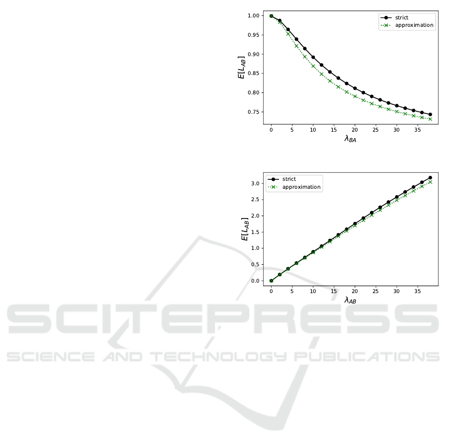
Figures 3 and 4 show the results for the number

of the waiting customers in class-AB (= E[L

]) ac-

cording to the values of λ

and λ

, respectively.

Overall, both solutions show a similar trend. The rea-

son why the heuristic solution is that we assume each

class’s independence. Therefore, it is easier to sat-

isfy the condition of CRS occurrences compared to

the theoretical solution, and thus, customers tend to

decrease quickly in the heuristic analysis. However,

it should be noted that the heuristic model has a much

smaller number of states (i.e., less memory capacity

required for the computation). We can consider that

the heuristic analysis is practical to obtain the rough

trend of the system performance with low computa-

tional cost.

6 CONCLUSION

This paper has considered the modeling of the intro-

duction of CRS (one of the demand-responsive trans

portations) on a circular bus route. First of all, we

have shown the theoretical analysis of the model re-

garding queueing theory. However, the theoretical

model is not practical from the perspective of its com-

putational cost. Therefore, we have proposed the

heuristic analysis, which estimates the steady state

probabilities algorithmically. We have conﬁrmed the

validity of the heuristic analysis compared to the theo-

retical analysis by conducting some numerical exper-

Figure 3: The expected number of the waiting customers.

Figure 4: The expected number of the waiting customers.

iments. As future works, we plan to conduct numeri-

cal experiments for more various cases, e.g., the case

where the number of nodes is more than 3. Moreover,

it is also an important issue that we conﬁrm the guar-

antee of the theoretical convergence of the heuristic

model.

ACKNOWLEDGEMENTS

This work is partly supported by JSPS KAKENHI

Nos. 19K12198, 18K18006, JST MIRAI No. JP-

MJMI19B1. This study is (partially) supported by

FMIRAI: R&D Center for Frontiers of MIRAI in Pol-

icy and Technology, the University of Tsukuba and

Toyota Motor Corporation collaborative R&D center.

REFERENCES

Agatz, N., Erera, A., Savelsbergh, M., and Wang, X. (2012).

Optimization for dynamic ride-sharing: a review. Eu-

ropean Journal of Operational Research, 223(2):295–

303.

Ando, H., Takahara, I., and Osawa, Y. (2019). Mobility

services in university campus. Communications of

ICORES 2022 - 11th International Conference on Operations Research and Enterprise Systems

198

the Operations Research Society of Japan, 64(8):447–

452.

Correia, G. and Antunes, A. (2012). Optimization approach

to depot location and trip selection in one-way car-

sharing systems. Transportation Research Part E,

48:233–247.

Daganzo, C. and Ouyang, Y. (2019). A general model of

demand-responsive transportation services: from taxi

to ride sharing to dial-a-ride. Transportation Research

Part B, 126:213–224.

Enzi, M., Parragh, S., Pisinger, D., and Prandtstetter, M.

(2021). Modeling and solving the multimodal car-and

ride-sharing problem. European Journal of Opera-

tional Research, 293(1):290–303.

Nakamura, A., Phung-Duc, T., and Ando, H. (2020a).

Queueing analysis for a mixed model of carsharing

and ridesharing. Lecture Notes in Computer Science,

LNCS 12023:42–56.

Nakamura, A., Phung-Duc, T., and Ando, H. (2020b). A

stochastic model for car/ride-share service by a bus

company. In Proceedings of The 2020 International

Symposium on Nonlinear Theory and Its Applications,

pages 312–315.

Tao, S. and Pender, J. (2020). A stochastic analysis of bike

sharing systems. Probability in the Engineering and

Informational Sciences, pages 1–58.

Queueing Model of Circular Demand Responsive Transportation System: Theoretical Solution and Heuristic Solution

199