Vectorization of Bias in Machine Learning Algorithms

Sophie Bekerman

1,∗ a

, Eric Chen

1,∗ b

, Lily Lin

2,∗ c

and George D. Monta Nez

1 d

AMISTAD Lab, Dept. of Computer Science, Harvey Mudd College, Claremont, CA, U.S.A.

Department of Math and Computer Science, Biola University, La Mirada, CA, U.S.A.

Keywords:

Inductive Bias, Algorithmic Bias, Vectorization, Algorithmic Search Framework.

Abstract:

We develop a method to measure and compare the inductive bias of classiﬁcations algorithms by vectorizing

aspects of their behavior. We compute a vectorized representation of the algorithm’s bias, known as the in-

ductive orientation vector, for a set of algorithms. This vector captures the algorithm’s probability distribution

over all possible hypotheses for a classiﬁcation task. We cluster and plot the algorithms’ inductive orientation

vectors to visually characterize their relationships. As algorithm behavior is inﬂuenced by the training dataset,

we construct a Benchmark Data Suite (BDS) matrix that considers algorithms’ pairwise distances across many

datasets, allowing for more robust comparisons. We identify many relationships supported by existing litera-

ture, such as those between k-Nearest Neighbor and Random Forests and among tree-based algorithms, and

evaluate the strength of those known connections, showing the potential of this geometric approach to investi-

gate black-box machine learning algorithms.

1 INTRODUCTION

With the growing prevalence of black-box algorithms

in machine learning, ﬁnding ways to evaluate these

algorithms is crucial. We propose the inductive orien-

tation vector, a geometric representation of bias, as a

tool for analyzing learning algorithms. The inductive

orientation vector captures the probability distribution

of an algorithm’s predictions. This vector originates

within the algorithmic search framework (Monta

nez

et al., 2019), and quantiﬁes the structural manifesta-

tions of various assumptions contained in general al-

gorithms. By empirically estimating this vector for

various algorithms, researchers can compare the al-

gorithms’ inductive biases on particular benchmark

datasets, much like how current model comparisons

use accuracy, precision, and memorization capacity

to compare algorithms (Caruana and Niculescu-Mizil,

2006; Osisanwo et al., 2017; Rong et al., 2021). In

doing so, we can identify hidden connections between

algorithms. By comparing the biases of new algo-

rithms to known biases of existing algorithms, we

provide a point of reference useful for determining

https://orcid.org/0000-0001-6497-3133

https://orcid.org/0000-0002-0469-3858

https://orcid.org/0000-0003-2500-6495

https://orcid.org/0000-0002-1333-4611

∗

These authors contributed equally

whether the new algorithms share signiﬁcant biases

with previous ones or incorporate novel assumptions.

We can also use the inductive orientation vector to

compute other algorithm quantities such as algorith-

mic bias (Bashir et al., 2020), algorithmic capacity,

and entropic expressivity (Lauw et al., 2020), which

we will explore in future work. The inductive orien-

tation vector provides an objective measure for bias

in black-box algorithms, making it easier to choose

the best algorithm for a problem without resorting to

heuristics. Previously a strictly theoretical concept,

this analysis allows us to evaluate the behavior of al-

gorithms without knowing its underlying structure.

The remainder is organized as follows. In Section

2, we discuss prior work related to bias and vector-

ization. In Section 3, we summarize the algorithmic

search framework and several relevant deﬁnitions. We

then establish a process to estimate inductive orienta-

tion vectors and present results in Section 4. In Sec-

tions 5 and 6, we implement and discuss additional

ways to analyze inductive orientation vectors.

2 RELATED WORK

The goal of the inductive orientation vector is to cap-

ture inductive bias. An algorithm’s inductive bias

is the set of assumptions the algorithm makes be-

354

Bekerman, S., Chen, E., Lin, L. and Monta Nez, G.

Vectorization of Bias in Machine Learning Algorithms.

DOI: 10.5220/0010845000003116

In Proceedings of the 14th International Conference on Agents and Artiﬁcial Intelligence (ICAART 2022) - Volume 2, pages 354-365

ISBN: 978-989-758-547-0; ISSN: 2184-433X

yond strict consistency with training data (Mitchell,

1980). This bias inheres in the algorithm, so it is

distinct from bias in the training data. Bias is nec-

essary for learning because, without it, a classiﬁca-

tion algorithm cannot generalize beyond training data

(Mitchell, 1980). This result has been supported ex-

perimentally (Runarsson and Yao, 2005), and for-

mally extended to show that algorithms must incor-

porate biasing assumptions to perform better than

uniform random guessing on unseen data (Monta

nez

et al., 2019). If inductive bias is responsible for an al-

gorithm’s successes and failures on various problems,

then algorithms with similar inductive biases may be-

have similarly on a greater proportion of problems

than algorithms with different biases. This predictive

potential of inductive biases motivates the concept of

the inductive orientation vector.

A vector representation of bias can allow geo-

metric analysis of hidden connections between var-

ious algorithms. Over the past decade, vectoriza-

tion has revolutionized machine learning. One promi-

nent case is vector space word embeddings in nat-

ural language processing. Word embedding meth-

ods capture semantic notions geometrically (Gonen

and Goldberg, 2019), allowing for “vector arithmetic”

of words, such as Madrid - Spain + France =

Paris (Mikolov et al., 2013). They are also useful in

practice: using word embeddings, the language model

GPT-3 recently achieved state-of-the-art results for

many natural language benchmark tasks (Brown et al.,

2020). Given the ubiquity and utility of vector repre-

sentations of words, a vector representation of bias

could be equally far-reaching.

3 THE SEARCH FRAMEWORK

3.1 The Search Problem

Inductive orientation vectors were initially introduced

in the context of the algorithmic search framework,

a learning-theory framework for analyzing machine

learning and search algorithms (Monta

nez, 2017). In-

ductive orientation vectors were designed to compute

speciﬁc theoretical quantities related to learning algo-

rithm performance; estimating these vectors empiri-

cally can allow us to estimate those related quantities

(Monta

nez et al., 2021). Within this framework, the

process of learning is cast as a search for an ideal hy-

pothesis (or hypotheses). Each search problem is rep-

resented by the 3-tuple, (Ω, T , F). The search space

Ω is a ﬁnite set of all possible solutions (hypotheses)

to a search problem. Within the set Ω is the target

set T that contains the desirable and/or acceptable so-

lutions. The target function t conveniently encodes

the relation between the target set and its respective

search space as a binary |T |-hot vector of length |Ω|.

Each entry in the target vector corresponds to a po-

tential solution ω in the search space. At each in-

dex, the target vector takes on the value of 1 if ω ∈ T

and 0 otherwise. The external information resource

F provides initialization information (e.g., training

data) and guides the algorithm in the search process

by evaluating elements of the search space (through

a loss or ﬁtness function). The search framework ac-

commodates many types of algorithms; for example,

we can cast classiﬁcation problems as search prob-

lems in the framework by considering classiﬁcation

as the search for a correct sequence of labels in the

search space of all possible labels (Monta

nez, 2017).

To make this more concrete, consider a classiﬁ-

cation problem in which there are C different labels

(classes). We train a classiﬁcation model on a training

set and evaluate its performance on a holdout (test) set

of size N. Here, we are searching for a correct (or ac-

ceptable) labeling of the entire holdout set; thus, the

search space Ω would be the set of all possible com-

binations of labeling the elements in the holdout set

where |Ω| = C

. The target set T would consist of

sequences of correct (or acceptable) labelings of the

holdout set. Depending on the problem, we might re-

quire that a sequence of labels be completely correct

to be included in the target set, or we might be satis-

ﬁed with sequences that label the holdout set within a

chosen threshold of accuracy. Finally, the external in-

formation resource F is the classiﬁcation model’s loss

function and data used to train the model.

3.2 The Search Algorithm

During the search process, a search algorithm A will

induce a probability distribution P

on the search

space Ω; the algorithm will assign higher probabil-

ity to elements in the search space that it perceives

are likely to be in the target set. The search process

is an iterative process; the number of iterations varies

depending on the learning task. For each iteration, the

search algorithm induces a probability distribution P

over the search space Ω which is determined using

the search history H. H contains a series of tuples

(ω

, F(ω

)) where ω

is a solution previously queried

by the algorithm at the ith iteration (or time step) and

its corresponding evaluation under the external infor-

mation resource F. At each iteration i an algorithm

queries an element ω

from the search space based

on the current probability distribution P

, evaluates

using the F, and adds the tuple (ω

, F(ω

)) into

the search history H. The algorithm then adjusts the

Vectorization of Bias in Machine Learning Algorithms

355

BLACK-BOX

ALGORITHM

HISTORY

ω₀, F(ω₀)

ω₃, F(ω₃)

ω₈, F(ω₈)

ω₅, F(ω₅)

ω₂, F(ω₂)

i − 6

i − 5

i − 4

i − 3

i − 2

i − 1

ω₆, F(ω₆)

CHOOSE NEXT POINT AT TIME STEP i

ω, F(ω)

Figure 1: Black-box search algorithm. At time i the algo-

rithm computes a probability distribution P

over the search

space Ω, using information from the history, and a new

point is drawn according to P

. The point is evaluated us-

ing external information resource F. The tuple (ω,F(ω)) is

then added to the history at position i. Note, indices on ω

elements do not correspond to time step in this diagram, but

to sampled locations.

probability distribution on the search space, P

i+1

, ac-

cording to the search history. By the end of a search

process (or run), a probability distribution sequence

P is produced. If, at the end of the run, the search

history contains at least one element in the target set,

the algorithm is successful; this is only evaluated after

the search process is completed because the algorithm

does not have access to the target set. Figure 1 pro-

vides a graphical representation of the search process.

3.3 Inductive Orientation Vector

Following Monta

nez, we use the expected per-query

probability of success to measure an algorithm’s per-

formance (Monta

nez, 2017). Per-query normaliza-

tion accounts for differences in the number of sam-

pling steps (iterations) per run. Taking the expectation

of multiple runs of the search process when trained

on the same information resource F accounts for any

stochastic differences between different runs. Mathe-

matically, the expected per-query probability of suc-

cess is deﬁned as

q(T, F) = E

P,H

∑

i=1

(ω ∈ T )



(1)

where

P is a sequence of probability distributions P

at each iteration i over the search space, T is the tar-

get set, F is the external information resource, and

H is the search history. The number of queries made

during a search is equal to the length of |

P|. The ex-

pectation accounts for stochastic differences between

multiple runs of the algorithm, while the inner quan-

tity measures the expected probability of success of a

single run (Lauw et al., 2020).

Previously, Monta

nez demonstrated a more con-

venient way of expressing the expected per-query

probability of success as the inner product of the tar-

get function and a vector representing the expected

probability distribution induced by the search algo-

rithm A over multiple runs (Monta

nez, 2017). Let P

be the vector representation of this averaged probabil-

ity distribution (conditioned on F) induced on Ω over

multiple runs of the search process. Formally, deﬁne

:= E

P,H

∑

i=1



. (2)

This is the inductive orientation vector of A relative

to a particular information resource F. The sum of

all the probability mass on elements in the target set

yields the probability of success, which is the prob-

ability that the algorithm queries an element in T .

This sum, known as the single-query probability of

success, is represented by t

, where t is a |T |-hot

target function. This establishes the equivalence be-

tween the expected per-query probability of success

over an entire search and the single-query probabil-

ity of success (sampled from the averaged probability

distribution induced by the search algorithm A in ex-

pectation), which is represented by q(T, F) = t

In the case that an algorithm is trained on different

information resources F, its expected performance is

calculated by ﬁnding an inductive orientation vector

relative to a data-generating distribution D on the

space of information resources F . Formally,

= E





= E

P,H

∑

i=1



(3)

where F is distributed according to D (i.e., F ∼ D).

Then, the expected per-query probability of success

of an algorithm A when trained on information re-

sources F generated by the data generating process D

is E

F∼D

[q(T,F)] = t

. Both measures of success,

q(T, F) and E

F∼D

[q(T,F)], will be used.

3.4 Inductive Bias

Since an inductive orientation vector represents a

learning algorithm’s probability distribution over its

search space, it captures aspects of the algorithm’s in-

ductive bias. Inductive bias is set of the assumptions

built into a model, implicitly or explicitly, that allow

it to generalize from training data. Although an algo-

rithm’s inductive bias determines how it interacts with

data, it is a property of the algorithm that is indepen-

dent of the data. However, the close relationship of

inductive bias and data makes it difﬁcult to isolate an

ICAART 2022 - 14th International Conference on Agents and Artiﬁcial Intelligence

356

algorithm’s inductive bias. Thus, the inductive orien-

tation vector, P

, aims to estimate this property rela-

tive to a speciﬁc distribution of information resources

and search space. When comparing the inductive ori-

entation vectors of different algorithms trained on the

same set of information resources and search space,

we can attribute their differences to differences be-

tween algorithms’ inductive biases. In this way, the

inductive orientation vector makes an algorithm’s as-

sumptions explicit and measurable.

4 ESTIMATING INDUCTIVE

ORIENTATIONS

4.1 Method

We now present our method for estimating induc-

tive orientation vectors. We begin by describing our

data-generating process as well as some alternative

methods, introducing the Labeling Distribution Ma-

trix, and reviewing the inductive orientation vector.

Given a dataset, we ﬁrst split the dataset into a

training set of n instances and a holdout set of size N.

Note that we assume this dataset to be representative

of its data-generating distribution D. To generate a

data resource F from the space, we sample a size m

subset from the size n training set with replacement

between subset selections. Note that each instance in

subset F is drawn without replacement.

Since F is a subset of the training set that was

drawn from D, F itself approximates a sample from

D (assuming m is large enough), being a subset of the

original i.i.d. instances drawn from that distribution.

Sampling m out of n instances is crucial, as this al-

lows us to estimate P

vectors even when we have

more data than is computationally feasible for train-

ing an algorithm. Each bootstrap subsample is drawn

from the empirical distribution which assigns to each

instance in the training dataset a probability of 1/n.

Having described our data-generating process, we

provide the pseudocode (Algorithm 1) of how we gen-

erate a Labeling Distribution Matrix (LDM, ﬁrst in-

troduced by (Sandoval Segura et al., 2020)) relative

to a learning algorithm A and a distribution D. We

introduce LDMs as they are our data structure for esti-

mating inductive orientation vectors. Before explain-

ing the details of this estimation, let us review how to

construct an LDM and what its components are.

Let K be the number of independently selected

subsets F of the training set. Let R be the number of

times we repeat the process of training A on the same

subsample F

; this is to account for the stochastic na-

ture of some algorithms. We let P

denote the aver-

Algorithm 1: Labeling Distribution Matrix (LDM).

1: for all k = 1,.. .,K do

2: F

← Sample without replacement from training set

3: for all r = 1,. .., R do

4: Generate P

after training A on F

5: P

= P

+ P

6: end for

7: P

= P

/ R

8: Store P

in LDM

9: end for

10: Return LDM

aged probability distribution induced over its search

space Ω after training A on the subsample F

R times.

Together, the K simplex vectors P

form the columns

of the LDM. Note that P

is the probability distribu-

tion vector averaged over only the ﬁnal iteration of

the search. In other words, P

corresponds to the

probability distribution induced over Ω at the last it-

eration in the search after being trained on F

. Having

computed the LDM, we compute the inductive orien-

tation vector P

relative to an algorithm A by simply

taking the average across the columns of the LDM.

In other words, we take the average of the P

’s to

be the inductive orientation vector relative to the data

distribution D (using our bootstrapped approximation

of it). In cases where multiple i.i.d. samples can be

drawn from D directly, the estimation will become

correspondingly more accurate.

4.1.1 Experimental Setup

To estimate inductive orientation vectors, we se-

lected a variety of machine learning algorithms from

Python’s scikit-learn library (version 0.22.2.post1)

(Pedregosa et al., 2011). The algorithms, along with

their parameters, are speciﬁed in Table 2. If a param-

eter is not speciﬁed, then the default value is used.

Note that both Linear SVC and SVC with a linear ker-

nel are included because we wanted to see if differ-

ences in implementation would affect algorithm be-

havior; Linear SVC is implemented using liblinear

rather than libsvm, making it more scalable for larger

datasets. Also, SGD Classiﬁers refer to algorithms

that are optimized by stochastic gradient descent. We

selected well-studied algorithms to evaluate our re-

sults against existing research. In general, our meth-

ods could be applied to any classiﬁcation algorithm.

Since inductive orientation vectors are relative to

an algorithm A and a data distribution D, we se-

lected 10 datasets, 9 of which were chosen from the

UCI Machine Learning Repository (Dua and Graff,

2017; Moro et al., 2014; Cortez et al., 2009; Baati

Vectorization of Bias in Machine Learning Algorithms

357

and Mohsil, 2020; Palechor and de la Hoz Manotas,

2019). One dataset (denoted Random dataset) was

generated using np.random with RandomState set to

42. These datasets were chosen with the intention of

having a collection of data of varying complexities to

test the strength of inductive orientation similarities

across diverse datasets. All datasets contain at least

1000 instances. For some datasets, feature engineer-

ing was used to encode categorical features as either

numerical values or one-hot vectors. To shorten the

estimation time for the inductive orientation vectors,

non-binary classiﬁcation datasets were converted into

binary classiﬁcation problems in a way that balanced

the number of instances in each class.

Table 1: Datasets, their sizes, the size m of the subset used to

train the learning algorithms, and dataset complexity ratios

(CR, described in the main text).

Dataset Size m CR

Obesity 2111 211 0.081

Letter Recognition 1609 260 0.254

Wine Quality 6496 500 0.345

Abalone 4176 417 0.747

Shopper’s Intention 12245 600 0.769

EEG Eye State 14980 600 0.780

Car Evaluation 1728 170 0.916

Bank Marketing 11162 500 0.980

Random 1609 260 1.004

Spam 4601 460 1.073

For each of the 10 datasets and for each algo-

rithm selected, we estimated the corresponding induc-

tive orientation vector using the following scheme: a

holdout set of 5 instances, 800 subsets sampled from

the training set (using the process outlined in Section

4.1), and 20 runs on the same data subset; namely,

N = 5, K = 800, and R = 20. Empirically, we found

that using 800 subsets led to more stable inductive

orientation vectors with low variance, and increasing

the number of subsets further did not signiﬁcantly de-

crease variance. For a given dataset, all algorithms

were trained on a subset of the data of the same size.

The size of the training subset depends on the dataset

(refer to Table 1 for details). For smaller datasets, the

number of instances per subset was reduced to avoid

signiﬁcant overlap between subsets.

We measured each dataset’s complexity by com-

puting the ratio of the average Euclidean distance be-

tween a point and its nearest neighbor of the same

class to the average distance between a point and its

nearest neighbor of a different class, as shown in Ta-

ble 1. A lower ratio suggests the dataset is more struc-

tured and likely to be separable with a simple decision

boundary. A higher ratio means the relationships be-

tween different classes are more complex. For large

datasets, it is computationally expensive to compute

the distance between every point, so a random sub-

sample of 6,900 elements was used. Further discus-

sion of this estimate of data complexity can be found

in other sources (Rong et al., 2021) and Section 4.2.

4.2 Results and Discussion

We now present results regarding the basic character-

istics of inductive orientation vectors as well as some

analysis of their values. For a depiction of the induc-

tive orientation vectors relative to the Bank Marketing

dataset, refer to Figure 2.

Inductive orientation vectors can differ greatly be-

tween datasets and between algorithms. For exam-

ple, the inductive orientation vectors relative to the

datasets Car Evaluation, Letter Recognition, Obesity,

and Wine Quality are more sparse than those relative

to Abalone, Bank Marketing, EEG Eye State, Ran-

dom, and Shopper’s Intention. This sparseness oc-

curs when an algorithm consistently predicts the same

element in Ω even when trained on different subsets

of the original training data. An algorithm that pre-

dicts in a similar manner across varying training sub-

sets suggests that the algorithm is able to generalize

to data outside its training subset, since each training

subset is randomly generated and typically different.

Sparse inductive orientation vectors tend to corre-

spond with datasets of lower complexity (cf. Table 1).

This trend suggests algorithms do not capture the gen-

eral trends in the data for datasets of high complex-

ity, leading to more varied predictions and a spread

out probability distribution. While this trend gener-

ally holds true, there are some deviations. For exam-

ple, while the dataset Spam has a complexity ratio of

1.073 (which exceeds even the Random dataset), its

inductive orientation vectors are more sparse than that

of Random. This is most likely because the complex-

ity ratio is not a perfect measure of dataset complex-

ity. The same can be said for the spareness of induc-

tive orientation vectors relative to the Car Evaluation

dataset. Based on this ratio, points in the dataset Spam

are closer to points of a different class than points of

the same class. Even so, a relationship could still be

detected in the data, causing the vectors to be more

sparse than those of the Random dataset. A randomly

generated dataset, however, clearly has no existing

pattern, so its inductive orientation vectors are uni-

form. Since most other datasets match our expecta-

tions, we generally attribute sparseness in inductive

orientation vectors to lower complexity in datasets.

We also conﬁrm that different instances of the

same algorithm typically have closely related induc-

tive orientation vectors, despite having different hy-

ICAART 2022 - 14th International Conference on Agents and Artiﬁcial Intelligence

358

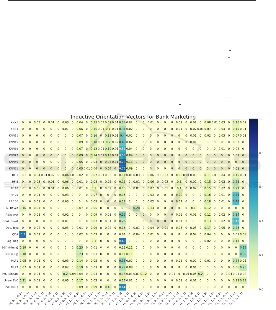
Table 2: Machine learning algorithms and their parameters. Note that SGD Classiﬁers refer to classiﬁers that are optimized

by Stochastic Gradient Descent. The base algorithm of SGD (Hinge) Classiﬁer is a linear support vector machine and that of

SGD (Log) is logistic regression.

Algorithm Name Abbreviation Hyperparameters

Adaboost Adaboost

Decision Tree Dec. Tree

Gradient Boosting Grad. Boost.

k-Nearest Neighbors KNN n neighbors (k): 1, 3, 11, 15,

19, 25, 49, 51

Logistic Regression Log. Reg. max iter:2000

Multi-layer Perceptron MLP(1,3) max iter:2000,

hidden layer sizes:(100), (150,100,50)

Guassian Naive Bayes N. Bayes

Quadratic Discriminant Analysis QDA

Random Forest RF n estimators:1,5,10,25,100

Stochastic Gradient Descent Classiﬁer SGD (Hinge, Log) max iter:2000, loss:‘hinge’, ‘log’

Linear Support Vector Classiﬁer Linear SVC max iter:2000

Support Vector Classiﬁer SVC (Linear/RBF) max iter:2000, kernel:‘linear’, ‘rbf’

Figure 2: Inductive orientation vectors of algorithms trained on the Bank Marketing Dataset (Note that each 5-tuple corre-

sponds to a particular way of classifying the elements in the holdout set. Each 5-tuple is in the search space Ω).

Vectorization of Bias in Machine Learning Algorithms

359

Figure 3: Out-of-bag error of Random Forest decreases as

number of trees increase for the Bank Marketing Dataset.

perparameters. We see this with the P

vectors rel-

ative to the Bank Marketing dataset, with the excep-

tion of the SVCs. For example, KNNs and Random

Forests concentrate their probability mass on the la-

beling (0,1,1,1,0), SGD Classiﬁers concentrate their

probability mass on (1,1,1,1,1), and MLPs concen-

trate their probability mass on (0,1,1,1,0). Although

changing the hyperparameters does lead to changes in

the probability distribution over Ω, the overall shapes

of the distributions across different instances of the

same algorithm are relatively stable, which means

that P

vectors of instances of the same algorithm

are generally distinct from that of other algorithms.

This suggests that, in many cases, changing the hy-

perparameters of an algorithm may not fundamentally

change the algorithm.

Analyzing the P

vectors of KNN relative to the

Bank Marketing dataset, we notice a positive corre-

lation between the number of neighbors k and the

amount of probability mass concentrated at the label-

ing (0,1,1,1,0). As k increases from 1 to 51, the proba-

bility mass on (0,1,1,1,0) increases from 0.24 to 0.73,

which means that KNN becomes more consistent in

its predictions for larger values of k. This is because,

as KNN considers increasingly larger neighborhoods

of data to make its prediction, it becomes less affected

by changes in data as well as noise. Taken to the

extreme, when it considers the entire training subset

as its neighborhood, KNN will be biased towards the

majority class, if the KNN instance assigns uniform

weighting to each neighbor. In contrast, KNNs with

smaller values of k are highly sensitive to changes

in data, causing variations in their predictions. This

is reﬂected in the P

vectors of KNN1 and KNN3

whose probability mass are distributed more evenly

across Ω. These conclusions based on the inductive

orientation vectors conﬁrm that the choice of k plays

a key role in how KNN will perform given a dataset.

A similar trend can be seen with the P

vectors of

Random Forest. Random Forest builds a forest of de-

cision trees by selecting a random subset of training

features and a different bootstrap sample of the train-

ing data for every tree. Thus, between different runs

of Random Forest 1, which consists of only one tree,

the bootstrap sample and training features selected are

likely to differ, making the algorithm highly sensi-

tive to variations in data. However, as the number of

trees in a Random Forest model increases, it is able to

generalize better and, thus, predict more consistently.

From Figure 3, we see that the out-of-bag (OOB) er-

ror (a measure of accuracy of a Random Forest model)

decreases as the number of trees increases, indicating

that Random Forest models with more trees are more

accurate. This correlates with our observation of the

vectors that as the number of trees increases, Ran-

dom Forest concentrates increasingly more probabil-

ity mass on the label it believes is correct. Thus, the

inductive orientation vectors are consistent with ex-

isting knowledge of these algorithms and can provide

new insights for algorithms that are less well-studied.

5 CLUSTERING

5.1 Method

Examining and comparing inductive orientation vec-

tors can become difﬁcult and impractical when the

number of classes and/or holdout set size increases.

Thus, a more effective way of identifying similarities

between algorithms is by analyzing cluster plots.

Cluster plots are generated in three steps: clus-

tering, dimensionality reduction, and plotting. We

cluster at the original dimension R

to preserve re-

lationships between inductive orientation vectors. We

used Meanshift as our clustering algorithm, avoid-

ing the need to specify the number of clusters or

set any hyperparameters; using Scikit-learn’s defaults

(Pedregosa et al., 2011) generally produced clusters

consistent with our expectations. Another advantage

of Meanshift is its ability to handle high-dimensional

data using Locality Sensitive Hashing (Cui et al.,

2011) which may be useful when working with in-

ductive orientation vectors of higher dimensions, al-

though it was not used in this study. To visualize the

vectors, we reduce the vectors using Principal Com-

ponent Analysis (PCA) to two dimensions. We use

PCA instead of other dimensionality reduction meth-

ods, such as t-SNE and UMAP, because PCA is not

stochastic, making it simpler to analyze. Having re-

duced the vectors to two dimensions, we plot them

and label them according to how they were clustered

in the original dimension. Note that the resulting clus-

ters in the plots may diverge slightly from how we

ICAART 2022 - 14th International Conference on Agents and Artiﬁcial Intelligence

360

might cluster the vectors in two dimensions because

the clusters were ﬁrst formed in the original space.

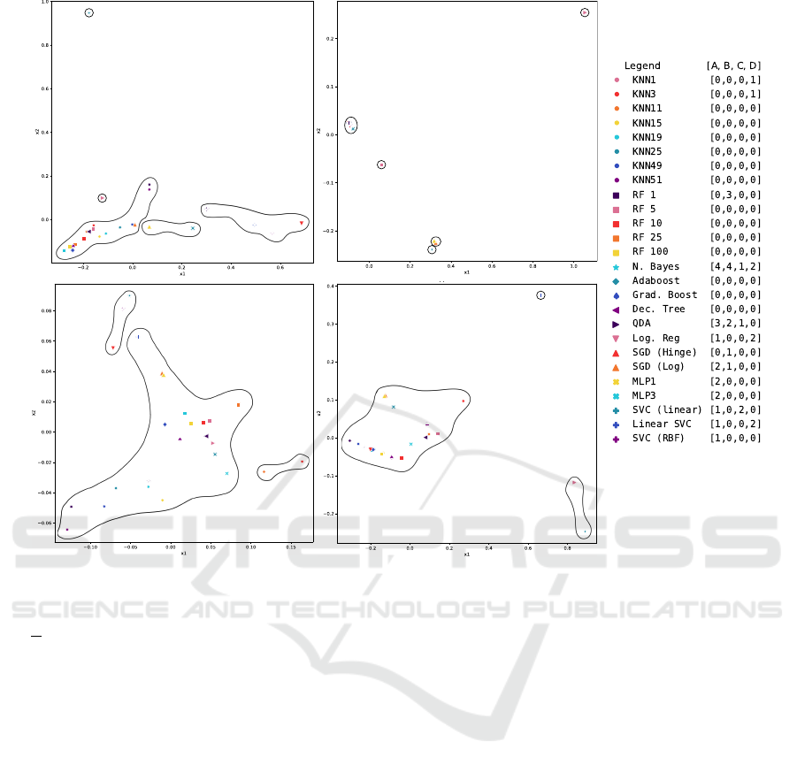
5.2 Results and Discussion

Across cluster plots, we observe that instances of

Random Forest, Decision Tree, Adaboost, and Gradi-

ent Boosting are consistently clustered together. This

is expected because these algorithms are all well-

known tree-based algorithms, extending and combin-

ing various implementations of decision trees. They

also all have axis-aligned decision boundaries, as seen

in Figure 5. Thus, it appears that similarities between

their inductive orientation vectors are a result of their

shared tree-based implementation. Furthermore, most

or all of the instances of the KNN and Random Forest

are clustered together in every plot. Existing research

supports this relationship, as Lin and Jeon classify

both algorithms as variants of weighted neighborhood

schemes (Lin and Jeon, 2006). In Figure 5, we also

see that they have somewhat similar decision bound-

aries. These ﬁndings suggest that cluster plots can un-

cover similarities between algorithms and, thus, are a

useful tool for directing further research.

We note that datasets with more structure like

Obesity and Letter Recognition have visually tighter

clusters, compared to unstructured datasets like Ran-

dom. Such analysis is limited since the scale of the

axes is generated by PCA for a speciﬁc collection of

inductive orientation vectors and, thus, not directly

comparable between plots.

6 BENCHMARK DATA SUITE

(BDS)

6.1 Method

While cluster plots are an effective way of visually

comparing inductive orientation vectors, the Bench-

mark Data Suite (BDS) matrix is a more precise com-

parison metric. This metric is based on pairwise

distances between inductive orientation vectors esti-

mated relative to the same dataset.

Deﬁnition 6.1 (Pairwise Distance). For a pair of in-

ductive orientation vectors P

D,A

and P

D,B

, the pair-

wise distance is the square of the Euclidean distances

between the vectors. Formally,

d(P

D,A

D,B

) =

|Ω|

∑

i=1

[i]

D,A

− P

[i]

D,B

)

(9)

where D is the data-generating distribution, i is the in-

dex, and |Ω| is the size of the search space and length

of the inductive orientation vector. Note that A and B

can be two separate learning algorithms or the same

learning algorithm with different parameterizations.

An algorithm’s BDS matrix is a matrix whose

columns are made up of pairwise distances between

the inductive orientation vector of the algorithm in

question and a set of learning algorithms all trained

on a particular dataset. The number of columns is

equal to the number of benchmark datasets, and each

column is relative to a different dataset. To balance

the inﬂuence of each dataset while preserving the rel-

ative distance between algorithms’ inductive orienta-

tion vectors for each dataset, we normalize each col-

umn of the BDS matrix by dividing by the corre-

sponding maximum pairwise distance. These scaling

factors are stored in a normalization vector. By multi-

plying the columns of a normalized BDS matrix with

its corresponding scaling factor in the normalization

vector, we can recover the unnormalized BDS matrix.

Given a set of learning algorithms A and a set of

datasets B, we present the following pseudocode to

ﬁnd the BDS of a ﬁxed algorithm A

∗

∈ A.

Algorithm 2: Benchmark Data Suite.

1: for all b ∈ B do

2: for all A ∈ A do

3: Compute the P

D,A

when trained on subsets of the

dataset b.

4: end for

5: for all A ∈ A \A

∗

6: Compute d(P

D,A

∗

) and insert into matrix.

7: end for

8: BDS ← Normalize the pairwise distances.

9: end for

10: Return BDS

6.1.1 Mean Pairwise Distance Vector

From the BDS matrix, we take the average across the

columns to produce a mean pairwise distance vector.

This aggregate vector reveals which relationships be-

tween inductive orientations hold across datasets and

which hold true for only a dataset. We sort this mean

distance vector by the average distance to more con-

veniently identify relationships between algorithms.

6.2 Results

Using the inductive orientation vectors presented in

Section 4.2, we generate mean pairwise distance vec-

tors for each of our algorithms.

The ﬁrst two columns of Table 3 show the sorted

mean pairwise distance vector of KNN11 which is

mostly representative of other instances of KNN. We

observe that, on average, the algorithms closest to

Vectorization of Bias in Machine Learning Algorithms

361

AbaloneA.

Obesity

RandomC.

Shopper’s Intention

Figure 4: Cluster plots of inductive orientation vectors using the Meanshift algorithm to cluster in the original dimensions and

PCA for dimensionality reduction. Boundaries around the plotted inductive orientations were added manually according to

the labels generated by Meanshift.

the P

of the KNN of interest are other instances

of KNN, speciﬁcally those with similar values of k.

Even so, not all instances of KNN may be close to

the KNN of interest. For example, KNN1 is one of

the furthest algorithms from KNN11. In general, in-

stances of KNN, Random Forest and other tree based

algorithms are the closest, followed by MLPs, and

then a mixture of SVCs and SGDs. The furthest algo-

rithms from KNN are QDA and Naive Bayes, which

we also observed in Section 5.2.

Considering Random Forest 100, we ﬁnd its near-

est algorithms are other instances of Random Forests

and Gradient Boosting. While both are types of boost-

ing, Gradient Boosting is consistently closer to in-

stances of Random Forest, excluding Random Forest

1, than Adaboost, suggesting greater similarities be-

tween the inductive biases of Gradient Boosting and

Random Forest. Of all instances of Random For-

est, Random Forest 1 is always furthest away from

the Random Forest of interest. This is likely because

Random Forest 1 makes its predictions based on a sin-

gle tree, unlike the other more extensive instances of

Random Forest. Besides a mixture of tree-based algo-

rithms, KNNs are relatively close, followed by MLPs,

Logistic Regression, and SVCs. Similar to the results

from KNN 11, QDA and Naive Bayes are the farthest

away from Random Forest 100. Although their mean

distance vectors are not shown, Adaboost and Gradi-

ent Boosting are closer to each other than to Random

Forest, likely because both are boosting algorithms.

Lastly, we notice that Naive Bayes, similar to SVC

with a linear kernel, is relatively far from all other al-

gorithms since the distances in the mean distance vec-

tor, on average, are much greater than those of other

algorithms. Of all algorithms, QDA’s inductive orien-

tation is most similar to that of Naive Bayes; even so,

their pairwise distance is still relatively large. Both

Naive Bayes and QDA are probabilistic models lever-

aging Bayes’ Theorem. However, Naive Bayes makes

an assumption that all input features are condition-

ally independent, while QDA does not. Essentially,

Naive Bayes is a simpliﬁed version of QDA (Ghojogh

and Crowley, 2019), which explains the large pair-

wise distance when the input features are correlated

and thus not conditionally independent.

ICAART 2022 - 14th International Conference on Agents and Artiﬁcial Intelligence

362

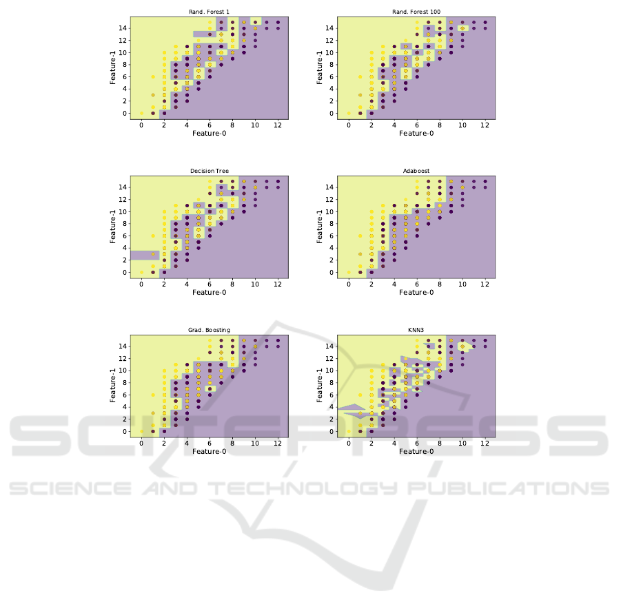
(a) Random Forest1. (b) Random Forest100.

(e) Gradient Boosting. (f) KNN3.

Figure 5: Example decision boundaries for two selected features for axis-aligned algorithms and KNN3. The data is generated

using the ﬁrst two features (x and y position of the box bounding the handwritten letter).

6.3 Discussion

Overall, the sorted mean pairwise distance vectors

match our conclusions from analyzing the raw induc-

tive orientation vectors and cluster plots. As men-

tioned previously, the mean distance vectors reveal

that different instances of the same algorithm tend to

be similar. Furthermore, cluster memberships are of-

ten reﬂected in the mean distance vectors. Most no-

tably, Naive Bayes and QDA, both of which are often

clustered on their own, also appear distant to other al-

gorithms according to the pairwise distance vectors.

Calculated based on pairwise distances, the mean

distance vector is limited in its ability to reﬂect

changes in how probability mass is distributed over

Ω. In Section 4.2, we noted an increase in the amount

of probability mass concentrated on a particular la-

beling as the number of neighbors (for KNN) and the

number of trees (for Random Forest) increased. This

trend, revealing how different hyperparameter values

affect the distribution over Ω, is difﬁcult to observe

when analyzing the sorted mean distance vector con-

sisting of only pairwise distances. For example, con-

sider again the mean distance vector of KNN11. Al-

though we can conclude that KNN15, KNN19, and

KNN25 are closer to KNN11 than KNN3, KNN49,

and KNN51, we are unaware of why instances of

KNN are not all close, in terms of pairwise distances.

On the other hand, if we examine the raw induc-

tive orientations, we see that, KNN49 and KNN51

concentrate more mass at (0,1,1,1,0) than KNN11,

whereas KNN3 has less. Furthermore, KNN1, ac-

cording to the mean distance vector, would be consid-

ered to be unrelated to KNN11 because its relation-

ship to KNN11 is overshadowed by its large pairwise

distance to KNN11. Thus, the mean distance vector

obscures some subtle patterns in the algorithms’ be-

havior. Even so, the limitations of mean pairwise vec-

tors can be overcome when used in conjunction with

cluster plots and analysis of the inductive orientation

vectors themselves.

Regardless, the mean distance vector is a power-

ful tool that provides a ranking of how similar other

algorithms are to an algorithm of interest based on

Vectorization of Bias in Machine Learning Algorithms

363

Table 3: Sorted mean pairwise distance vectors for KNN11, Random Forest 100, and Naive Bayes. Algorithms with smaller

distances are sorted to be near the top.

KNN 11 Random Forest 100 Naive Bayes

Algorithm Name d(P

) Algorithm Name d(P

)

KNN15 0.007 RF 25 0.007 QDA 0.272

KNN19 0.020 Grad. Boost. 0.038 RF 5 0.320

KNN25 0.037 RF 5 0.044 Linear SVC 0.344

RF 25 0.064 RF 10 0.053 MLP3 0.350

RF 5 0.072 KNN11 0.080 MLP1 0.353

RF 100 0.075 KNN15 0.082 SGD (Hinge) 0.360

Grad. Boost. 0.085 Adaboost 0.091 SGD (Log) 0.364

RF 10 0.098 KNN19 0.111 KNN11 0.365

Adaboost 0.102 Dec. Tree 0.126 RF 10 0.370

MLP1 0.115 KNN25 0.138 RF 25 0.374

KNN3 0.118 KNN3 0.143 KNN15 0.377

KNN51 0.119 MLP1 0.143 Dec. Tree 0.378

MLP3 0.123 MLP3 0.157 SVC (Linear) 0.379

KNN49 0.124 KNN51 0.227 KNN19 0.387

Dec. Tree 0.144 KNN49 0.239 Grad. Boost. 0.393

Log. Reg. 0.202 Log. Reg. 0.241 Adaboost 0.398

Linear SVC 0.233 Linear SVC 0.249 KNN3 0.402

SVC (RBF) 0.241 RF 1 0.253 KNN25 0.405

SGD (Hinge) 0.250 SGD (Hinge) 0.270 RF 100 0.409

SGD (Log) 0.251 SGD (Log) 0.272 RF 1 0.432

RF 1 0.262 KNN1 0.309 KNN51 0.446

KNN1 0.287 SVC (RBF) 0.309 KNN49 0.451

SVC (Linear) 0.362 SVC (Linear) 0.385 Log. Reg. 0.494

QDA 0.430 QDA 0.454 KNN1 0.502

N. Bayes 0.454 N. Bayes 0.463 SVC (RBF) 0.507

pairwise distances aggregated across datasets. Since

the inductive biases of algorithms are captured in their

respective inductive orientations (used in calculating

pairwise distances), the mean distance vector allows

us to gauge whether (and/or which) algorithms have

similar inductive biases as the algorithm of interest.

Accounting for all relationships across datasets, the

mean distance vector is a reliable and quantitative way

of comparing algorithms. This is because an algo-

rithm must be consistently close, in terms of pair-

wise distance, to the algorithm of interest across all

datasets for it to also be close in the resulting mean

distance vector. Additionally, connections between

algorithms, such as QDA and Naive Bayes, would be

difﬁcult to establish through a cluster plot, especially

since the coordinate distances between algorithms can

be distorted in the process of dimensionality reduc-

tion. These difﬁculties, however, are avoided when

using mean distance vectors.

Lastly, although not explored in-depth here, the

BDS matrix is a versatile tool of which many aspects

of the BDS matrix can be modiﬁed, namely, the nor-

malization method, set of benchmark datasets, set of

algorithms, aggregation method, and even the pair-

wise distance metric. In these ways, the BDS matrix

can be adapted for many other applications.

7 CONCLUSION

We develop a method to estimate the inductive ori-

entation vector of a classiﬁcation algorithm using a

modiﬁed Labeling Distribution Matrix (LDM). The

inductive orientation captures an algorithm’s induc-

tive bias relative to a certain dataset, providing an em-

pirical basis for algorithm comparison. These vectors

allow us to conﬁrm several known similarities among

existing algorithms, and this method therefore holds

promise for characterizing novel algorithms. Induc-

tive orientation vectors allow us to study the effects of

algorithm hyperparameterization in a consistent way

across algorithms. We explore inductive orientations

visually using cluster plots and numerically using the

Benchmark Data Suite, a particularly helpful foun-

dation for studying algorithmic relationships across

many diverse datasets.

Importantly, the LDM can used to calculate induc-

tive orientation vectors for arbitrary black-box classi-

ﬁcation algorithms. While our estimation procedure

was developed in this case for binary classiﬁcation

algorithms, regression and general search algorithms

also produce inductive orientation vectors (Monta

nez,

2017). Adapting these methods for non-classiﬁcation

algorithms is the subject of future work. By com-

ICAART 2022 - 14th International Conference on Agents and Artiﬁcial Intelligence

364

paring the biases of new algorithms to known biases

of existing algorithms, we can provide a point of ref-

erence for comparing algorithm biases and inductive

assumptions. Making biases explainable and measur-

able is of growing importance, given the increasing

use of complex, overparameterized models such as

deep neural networks. Inductive orientation vectors

provide a quantitative tool for measuring and compar-

ing inductive biases across algorithms.

ACKNOWLEDGEMENTS

This research was supported in part by the National

Science Foundation under Grant No. 1950885. Any

opinions, ﬁndings, or conclusions are those of the au-

thors alone, and do not necessarily reﬂect the views

of the National Science Foundation.

REFERENCES

Baati, K. and Mohsil, M. (2020). Real-Time Prediction

of Online Shoppers’ Purchasing Intention Using Ran-

dom Forest. In IFIP International Conference on Arti-

ﬁcial Intelligence Applications and Innovations, pages

43–51. Springer.

Bashir, D., Monta

nez, G. D., Sehra, S., Sandoval Segura,

P., and Lauw, J. (2020). An Information-Theoretic

Perspective on Overﬁtting and Underﬁtting. Aus-

tralasian Joint Conference on Artiﬁcial Intelligence

(AJCAI 2020).

Brown, T. B., Mann, B., Ryder, N., Subbiah, M., Kaplan, J.,

Dhariwal, P., Neelakantan, A., Shyam, P., Sastry, G.,

Askell, A., et al. (2020). Language Models are Few-

Shot Learners. arXiv preprint arXiv:2005.14165.

Caruana, R. and Niculescu-Mizil, A. (2006). An Empirical

Comparison of Supervised Learning Algorithms. In

Proceedings of the 23rd international conference on

Machine learning, pages 161–168.

Cortez, P., Cerdeira, A., Almeida, F., Matos, T., and Reis, J.

(2009). Modeling Wine Preferences by Data Mining

from Physicochemical Properties. Decision support

systems, 47(4):547–553.

Cui, Y., Cao, K., Zheng, G., and Zhang, F. (2011). An

Adaptive Mean Shift Algorithm Based on LSH. Pro-

cedia Engineering, 23:265–269.

Dua, D. and Graff, C. (2017). UCI Machine Learning

Repository.

Ghojogh, B. and Crowley, M. (2019). Linear and Quadratic

Discriminant Analysis: Tutorial. arXiv preprint

arXiv:1906.02590.

Gonen, H. and Goldberg, Y. (2019). Lipstick on a Pig: De-

biasing Methods Cover up Systematic Gender Biases

in Word Embeddings But do not Remove Them. arXiv

preprint arXiv:1903.03862.

Lauw, J., Macias, D., Trikha, A., Vendemiatti, J., and

Monta

nez, G. D. (2020). The Bias-Expressivity

Trade-off. In Proceedings of the 12th International

Conference on Agents and Artiﬁcial Intelligence - Vol-

ume 2, pages 141–150. SCITEPRESS.

Lin, Y. and Jeon, Y. (2006). Random Forests and Adaptive

Nearest Neighbors. Journal of the American Statisti-

cal Association, 101(474):578–590.

Mikolov, T., Sutskever, I., Chen, K., Corrado, G. S.,

and Dean, J. (2013). Distributed Representations of

Words and Phrases and their Compositionality. In

Advances in Neural Information Processing Systems,

pages 3111–3119.

Mitchell, T. M. (1980). The Need for Biases in Learning

Generalizations. Department of Computer Science,

Laboratory for Computer Science Research, Rutgers

Univ.

Monta

nez, G. D. (2017). The Famine of Forte: Few Search

Problems Greatly Favor Your Algorithm. In Systems,

Man, and Cybernetics (SMC), 2017 IEEE Interna-

tional Conference on, pages 477–482. IEEE.

Monta

nez, G. D., Bashir, D., and Lauw, J. (2021). Trad-

ing Bias for Expressivity in Artiﬁcial Learning. In

Agents and Artiﬁcial Intelligence, pages 332–353,

Cham. Springer International Publishing.

Monta

nez, G. D., Hayase, J., Lauw, J., Macias, D., Trikha,

A., and Vendemiatti, J. (2019). The Futility of Bias-

Free Learning and Search. In 32nd Australasian Joint

Conference on Artiﬁcial Intelligence, pages 277–288.

Springer.

Moro, S., Cortez, P., and Rita, P. (2014). A Data-Driven Ap-

proach to Predict the Success of Bank Telemarketing.

Decision Support Systems, 62:22–31.

Osisanwo, F., Akinsola, J., Awodele, O., Hinmikaiye,

J., Olakanmi, O., and Akinjobi, J. (2017). Super-

vised Machine Learning Algorithms: Classiﬁcation

and Comparison. International Journal of Computer

Trends and Technology (IJCTT), 48(3):128–138.

Palechor, F. M. and de la Hoz Manotas, A. (2019).

Dataset for Estimation of Obesity Levels Based on

Eating Habits and Physical Condition in Individuals

from Colombia, Peru and Mexico. Data in brief,

25:104344.

Pedregosa, F., Varoquaux, G., Gramfort, A., Michel, V.,

Thirion, B., Grisel, O., Blondel, M., Prettenhofer, P.,

Weiss, R., Dubourg, V., Vanderplas, J., Passos, A.,

Cournapeau, D., Brucher, M., Perrot, M., and Duch-

esnay, E. (2011). Scikit-learn: Machine Learning

in Python. Journal of Machine Learning Research,

12:2825–2830.

Rong, K., Khant, A., Flores, D., and Monta

nez, G. D.

(2021). The Label Recorder Method: Testing the

Memorization Capacity of Machine Learning Mod-

els. In The Seventh International Conference on

Machine Learning, Optimization, and Data Science

(LOD 2021).

Runarsson, T. P. and Yao, X. (2005). Search Biases in Con-

strained Evolutionary Optimization. IEEE Transac-

tions on Systems, Man, and Cybernetics, Part C (Ap-

plications and Reviews), 35(2):233–243.

Sandoval Segura, P., Lauw, J., Bashir, D., Shah, K., Sehra,

S., Macias, D., and Monta

nez, G. D. (2020). The

Labeling Distribution Matrix (LDM): A Tool for Es-

timating Machine Learning Algorithm Capacity. In

Proceedings of the 12th International Conference on

Agents and Artiﬁcial Intelligence - Volume 2, pages

980–986. SCITEPRESS.

Vectorization of Bias in Machine Learning Algorithms

365