The Comparison of Various Correlation Network Models in Studying

Mobility Data for the Analysis of Depression Episodes

Rama Krishna Thelagathoti

and Hesham H. Ali

College of Information Science and Technology, University of Nebraska Omaha, Omaha, NE 68182, U.S.A.

Keywords:

Depression, Mobility, Population Analysis, Correlation Network.

Abstract:

Depression is a serious mental health disorder affecting millions of people around the world. Traditional

diagnostic approaches are subjective including self-reporting feedback from patients and observational eval-

uation by a trained physician. However, altered motor activity is the central feature for depressive disorder.

Moreover, recent studies show that the analysis of motor activity is the best predictor in characterizing psycho-

logical disorders including depression. With the advent of wearable devices, an individual’s motor activity can

be monitored naturally using body worn sensors and feasible to distinguish depressed persons from healthy

individuals. In this manuscript, we hypothesis to apply a methodology that takes advantage of motor activity

recorded from wearable devices and process mobility patterns for a given group of subjects. Besides, em-

ployed a population analysis approach using correlation networks that evaluates mobility parameters of the

population and identify subgroups that exhibit similar motor complexity. We have analyzed the mobility data

of the given group by extracting three different sets of features using hour-wise, day-wise, and hybrid mobility

data. Also, a comparison study of three models is presented by constructing a correlation graph and ﬁnding

a cluster of individuals exhibiting similar mobility patterns. We found that mobility data using hour-wise

features provides the best results compared to the other two models.

1 INTRODUCTION

According to World Health Organization (WHO), ap-

proximately 280 million individuals suffer from de-

pression around the world which is equivalent to 3.8%

of the total world population (The World Health Or-

ganization(WHO), 2021). Moreover, depression may

impact any person regardless of their age, race, and

socio-economic background. However, it is likely

to affect adults than children. The onset of depres-

sion may not trigger by normal mood ﬂuctuations

or temporary emotional disturbance, rather when the

sadness becomes recurrent with intense severity that

leads to a major depressive disorder (Abuse, 2018).

Depression is a serious mental health condition that

may cause frequent mood swings which result in a

deprived quality of life. Furthermore, recent studies

show that there is a surge in suicides in depressed

patients due to feelings of loneliness (Curtin et al.,

2016). Depression often may inﬂuence the work-life

balance and cause poor performance in studies. It is

due to the symptomatic nature of illness which causes

https://orcid.org/0000-0002-4986-5027

https://orcid.org/0000-0002-8016-6144

a gloomy mind, lack of pleasure in doing routine ac-

tivities, feeling worthlessness, and hopelessness (The

National Institute of Mental Health (NIMH), 2021).

It is known that there is no precise pathology test

such as a blood routine test to accurately diagnose

depression, yet most of the existing clinical progno-

sis is largely dependent on visual observation. Nu-

merous subjective diagnostic scales were proposed

to measure the severity of the disease. For exam-

ple, the Center for Epidemiologic Studies Depres-

sion Scale (CES-D) is a self-reporting method that

measures the severity on a 4-point scale (Radloff,

1977). Similarly, the Montgomery-Asberg Depres-

sion Rating Scale (MADRS) measures the serious-

ness of the disorder on a 7-point scale which is ex-

clusively designed for adults over 18 years of age

(Montgomery and

Asberg, 1979). The drawback of

these approaches is that these methods merely de-

pend on human perception and comprehension skills.

Therefore, it is important to develop a sophisticated

methodology that is observer independent.

Although the main cause of depression is an ab-

normality in neurological functioning, altered motor

activity is one of the common symptoms that ap-

200

Thelagathoti, R. and Ali, H.

The Comparison of Various Correlation Network Models in Studying Mobility Data for the Analysis of Depression Episodes.

DOI: 10.5220/0010844500003123

In Proceedings of the 15th International Joint Conference on Biomedical Engineering Systems and Technologies (BIOSTEC 2022) - Volume 4: BIOSIGNALS, pages 200-207

ISBN: 978-989-758-552-4; ISSN: 2184-4305

pear in patients suffering from depression. Besides,

previous studies demonstrate that analysis of motor

skills is an important aid in classifying depressed pa-

tients from healthy counterparts (Sobin and Sackeim,

1997). Moreover, the depressed group compose lower

body reaction time and decreased body movements

than healthy persons. This opens a door for new pos-

sibilities to categorize depression by utilizing their

mobility data. Altered or lessened motor activity al-

lows to distinguish depressed patients from healthy

subjects. Proliferation in sensing technologies cre-

ated tiny wearable devices to record motor behavior

unobtrusively in a natural setting without disturbing

the daily activities. Wearable devices are proved to

be efﬁcient, affordable, unobtrusive, and more conve-

nient for they can even ﬁt a newborn child and collect

the data for several days (Heinze et al., 2010).

For our tests, we have chosen the ’Depresjon’

dataset downloaded from the public database (Garcia-

Ceja et al., 2018). It consists of 55 subjects catego-

rized into two groups: the ﬁrst group has 23 patients

diagnosed with either unipolar or bipolar depression

(the condition group) and the second group contains

32 healthy control subjects (the control group). The

main objectives of this study are as follows

1. Extracting three different categories of features

that represent motor activity segmented by the

hour, day, and combination of an hour as well as

day.

2. Employing the population analysis-based correla-

tion network approach to construct a graph where

the group of persons with similar mobility proﬁles

are strongly connected in the resultant graph.

3. Applying an appropriate clustering algorithm to

obtain potential subgroups in which each sub-

group represents a set of individuals exhibiting

similar motor complexity.

4. Comparison study of results obtained from three

different categories of features namely hour-wise,

day-wise, and hybrid.

The rest of the paper is organized as follows. Sec-

tion 2 covers the previous studies conducted on the

dataset. Section 3 describes a brief description of the

dataset, feature extraction, and correlation graph con-

struction. Whereas experimental results are shown in

section 4 and post hoc analysis of the obtained results

is elaborated in section 5.

2 RELATED WORK

In the past, several investigators have performed dif-

ferent experiments with the dataset. The dataset

was created by Garcia-Ceja et al. (Garcia-Ceja

et al., 2018) and published baseline performance re-

sults. They tested with different machine learning

algorithms but ﬁnally obtained higher accuracy of

73% with Linear Support Vector Machine (SVM).

In another research carried by Rodr

ıguez-Ruiz et al.

(Rodr

ıguez-Ruiz et al., 2020) processed motor data

and divided it into three sets as day, night, and full-

day activity data. The fundamental objective of this

work is to compare the motor activity patterns across

three different times of a day and draw profound in-

sights. They concluded that the features used to build

the nighttime motor data produced promising results

compared to the other two features. They obtained the

highest sensitivity and speciﬁcity of 99.4% and 99.9%

respectively.

On the other hand, Zanella-Calzada et al.

(Zanella-Calzada et al., 2019) extracted hour-wise

features by segmenting the overall motor activity into

the one-hour interval, trained the model using a Ran-

dom Forest classiﬁer. Their model achieved 87% ac-

curacy while the sensitivity was 87% and speciﬁcity

was 92% . Similarly, Galvan-Tejada et al. (Galv

an-

Tejada et al., 2019) mined 38 statistical features be-

longing to the time and frequency domain. They have

employed a genetic algorithm-based feature selection

approach to identify the best features. They also used

Random Forest to predict between healthy and de-

pressed and obtained a sensitivity of 68% and a speci-

ﬁcity of 61% .

Most of the researchers applied machine learning

techniques such as Random Forest and support vector

machines. Furthermore, they analyzed the data by us-

ing supervised machine learning methods by adding

a class label manually for each subject (0/YES for

condition group and 1/NO for control group or vice

versa). The novelty of our approach is that we do not

include known labels in the study, but we identify the

group of subjects by utilizing their mobility. In such

groups, condition subjects are gathered into a single

cluster and control subjects into another cluster.

3 MATERIALS AND METHODS

3.1 The Pipeline

Fig. 1 depicts the processing pipeline for correlation

graph analysis for mobility data acquired from De-

pressed patients. In the ﬁrst step, a dataset is acquired

from the public repository. In the preprocessing step,

data is cleaned, normalized, and eliminated outliers.

In the third step, three different types of features are

extracted namely hour-wise (Model M1), day-wise

The Comparison of Various Correlation Network Models in Studying Mobility Data for the Analysis of Depression Episodes

201

Figure 1: The pipeline for correlation network model.

(Model M2), and hybrid (Model M3). The models

M1, M2, and M3 represent the average motor activity

data segmented by the hour, day, and the combina-

tion of an hour as well as day respectively. Then, a

pair-wise correlation is applied for each of the mod-

els to construct a correlation graph. Then, strongly

connected clusters are detected from the correlation

graph. Finally, resultant graphs are analyzed and dis-

cussed

3.2 Dataset Description

In this study, we have used the ’Depresjon’ dataset

(Garcia-Ceja et al., 2018). It is a public dataset con-

sisting of motor activity collected from 55 partici-

pants including 23 persons belonging to the condi-

tion group and 32 subjects belonging to the control

group. The persons in the condition group were di-

agnosed with either unipolar or bipolar disorder and

they are under antidepressant medications. Whereas

the 32 participants in the control group are healthy

individuals. In this document, motor activity data

and mobility data are used interchangeably through-

out this document. Their motor activity was recorded

using a body-worn wearable sensor embedded in an

Actigraph watch (Name: Actiwatch, Manufacturer:

Cambridge Neurotechnology Ltd, England, Model

AW4). For the comfort of all participants, the acti-

graph watch was worn on the right wrist and their mo-

bility data was continuously monitored in the natural

environment. None of the participants were called to

a pathology lab or followed any speciﬁc instructions.

The actigraph measures the activity with a piezoelec-

tric accelerometer that is designed to record the in-

tensity, quantity, and duration of movement in all di-

rections. The Motion data was captured with a sam-

pling frequency of 32Hz and movements over 0.05g

for every minute in the form of activity count. The

actigraph records the motor activity in the form of an

activity count. The higher activity count resembles

the higher intensity in the motor activity.

The captured mobility data contains activity count

along with its timestamp. Besides, each participant’s

mobility data was stored in a separate data ﬁle, and

they can be identiﬁed with a unique contributor id.

Moreover, all of them were participated and provided

their data for a different number of days. However, on

average every person has 12 days of motor activity.

In addition to the data ﬁle, individuals’ demographic

characteristics are provided in a separate ﬁle (scores

ﬁle). This ﬁle contains the important information of

each person such as person unique id, days (number

of days of data monitored), gender (1:female, 2:male),

age (age range), afftype (1: bipolar II, 2: unipolar

depressive, 3: bipolar I), melanch (1: melancholia,

2: no melancholia), In addition to this, every subject

in the condition group was assessed by MADRS ob-

servational scale (Montgomery and

Asberg, 1979) at

the start of the data collection and also at the end of

the data collection. The MADRS scores are available

under MADRS1 and MADRS2 columns respectively.

Further, a statistical summary of all 55 participants

and their demographic details are described in Table

3.3 Preprocessing

The ﬁrst step in preprocessing phase is combining the

individual raw sensor data into a single dataset and

preparing for further processing. The motor activity

data was not measured for the same duration. How-

ever, on average 12 days of motor data is available

for all the users. Furthermore, the number of days

the data is available is not consistent between the user

sensor data ﬁle and the scores ﬁle. Therefore, we have

Table 1: Demographic characteristics.

Condition group Control group

Statistic Mean SD Mean SD

Days 12.6 2.3 12.6 2.7

Age 42.8 11 38.2 13

MADRS 1 22.7 4.8

MADRS 2 20 4.7

Statistic Total % Total %

Gender (Male) 13 57 12 38

Depression

(Bipolar)

8 34

Hospitalized

(Inpatient)

5 22

BIOSIGNALS 2022 - 15th International Conference on Bio-inspired Systems and Signal Processing

202

Table 2: Model-wise features.

Model

name

Feature

name

Features

count

Feature description

M1:

Hour-

wise

model

m0-

m23

The Average motor ac-

tivity measured for every

hour for 0-23 hours

sd0-

sd23

The standard deviation of

motor activity measured

for every hour for 0-23

hours

M2:

Day-

wise

model

dm1-

dm19

The Average motor activ-

ity measured for each day

for 1-19 days

dsd1-

dsd19

The standard deviation of

motor activity measured

for each day for 1-19 days

M3:

Hy-

brid

model

m0-

m23

The Average motor ac-

tivity measured for every

hour for 0-23 hours

sd0-

sd23

The standard deviation of

motor activity measured

for every hour for 0-23

hours

dm1-

dm19

The Average motor activ-

ity measured for each day

for 1-19 days

dsd1-

dsd19

The standard deviation of

motor activity measured

for each day for 1-19 days

id 1

A unique id to represent

each subject

taken the number of days mentioned in the scores ﬁle

as the ground truth and deleted the additional days of

motor data present in the sensor data ﬁle for each par-

ticipant. In the next step, the activity signal is nor-

malized, and removed outliers. The activity signal

data is normalized between 0 and 1 using the Z-score

standardization technique. Since the condition and

control groups belong to two different entities, both

groups’ sensors data is normalized separately. In the

next step, outliers are eliminated by utilizing the in-

terquartile range (IQR) property. In this context, a

data point is considered an outlier if it is below the

ﬁrst quartile or above the third quartile. In this pro-

cess, outliers are not removed rather they are replaced

with either the ﬁrst quartile or the third quartile de-

pending on whether the data point is above the third

quartile or below the ﬁrst quartile respectively. The

resultant dataset is normalized and free from outliers.

3.4 Feature Extraction

Each participant has shared their mobility data for a

certain number of days. But all of them were not col-

lected their motor data for the same number of days.

For example, participant 8 in the condition group has

provided mobility data for 5 days, while person 2 has

20 days of motor data. In this manuscript, we propose

to utilize three different types of features: hour-wise

features (Model M1) that represent hourly motor ac-

tivity in a 24-hour cycle, day-wise features (Model

M2) that signiﬁes overall day motor activity, hybrid

features (Model M3) that combine both hour-wise and

day-wise features. The detailed list of features is elab-

orated in Table 2.

In the hour-wise model (M1), motor activity is

segmented by an hourly pattern. Although each par-

ticipant generated motor activity for a variable num-

ber of days, the total activity of a person for all days

is aggregated before extraction of the features. Then

each person’s motor data is divided by an hour inter-

val. Further, the mean and the standard deviation (SD)

are computed for every hour of aggregated data. As

a result, 24 features are generated from mean and an-

other 24 features are generated from SD. In the day-

wise model (M2), a person’s motor data of a day is

aggregated, and this process is repeated for all days.

Then mean and SD is calculated for each day. From

the dataset, it is known that each participant’s motor

activity is collected for a variable number of days, yet

a user has not more than 19 days of activity data. So,

19 features of as day-wise activity means, and 19 fea-

tures of day-wise SD are processed. This process pro-

duces 38 features for each person. Since every par-

ticipant does not possess 19 days of sensor data, the

remaining days where the data is not present are ﬁlled

with 0. To eliminate the bias of the number of days

between two persons, the minimum number of days

is considered during modeling. In the hybrid model

(M3), 48 features from the hour-wise model and 38

features from the day-wise model are combined. Ef-

fectively M3 model generates 86 features.

3.5 Construction of Correlation

Network Model

The objective of building a correlation graph is to

understand the interrelationships among the partici-

pants concerning their mobility parameters. In previ-

ous experiments (Garcia-Ceja et al., 2018) (Zanella-

Calzada et al., 2019), researchers have employed ma-

chine learning approaches and classiﬁed depressed

patients from the healthy control group. Neverthe-

less, all these studies have utilized a known class la-

bel such as 0/NO for healthy control subjects, 1/YES

for a depressed patient, then try to classify the sub-

jects and measure the accuracy of the prediction al-

gorithm. The inherent downside of this approach is

that the learning algorithm works only if the known

The Comparison of Various Correlation Network Models in Studying Mobility Data for the Analysis of Depression Episodes

203

label is present in the dataset. Besides, these method-

ologies are label-driven. In this manuscript, we intro-

duce a data-driven approach by employing a popula-

tion analysis approach using correlation graphs. This

approach does not require a label to be present in

the dataset rather it analyzes the mobility parameters

of the given group and identiﬁes the subgroups that

demonstrate similar mobility patterns. Our hypothe-

sis is developed on the fact that subgroups in the given

group compose similar motor activity which makes

them distinguishable from other groups. This is fur-

ther exempliﬁed from the motor data of 55 subjects

where the overall mean activity of the condition group

is 284 while the condition group has 187.

The ﬁrst step in the graph creation is to establish

the relationship between each pair of subjects with re-

spect to their motor activity data. Once the relation-

ships are identiﬁed, their interconnections are repre-

sented using a graph. A graph G = (V, E) is an ab-

stract mathematical representation of any system that

depicts the relationships between the objects. In such

a graph, nodes or vertices (V) denotes the elements

of the system, and edges (E) represent the intercon-

nection between the elements (Dongen, 2000). In this

study, all 55 participants are denoted as nodes, and

their relationship regarding their motor activity is rep-

resented as an edge. It implies that two participants

are connected by an edge if they possess a similar mo-

tor activity proﬁle.

The degree of similarity between each pair of sub-

jects is measured using the Pearson pair-wise correla-

tion coefﬁcient (ρ). The Pearson pair-wise correlation

coefﬁcient measures the linear dependence between

a pair of objects. Usually, the value ranges between

-1 and +1 where -1 indicates a negative correlation

and +1 signiﬁes a strong positive correlation. To con-

struct the correlation graph, the ρ value is computed

between each pair of users by utilizing their motor

activity data. This operation outputs a correlation ma-

trix with pair-wise correlation coefﬁcient values. The

ρ value between a pair of users signiﬁes the degree

of similarity with regards to their motor activity. The

higher the ρ value the stronger the relationship be-

tween the pair of users. To create the graph from the

correlation matrix, strongly correlated pairs are iden-

tiﬁed by using the signiﬁcance matrix. A signiﬁcance

matrix is obtained by setting a predeﬁned threshold k

using equation 1.

signiﬁcance matrix(i, j) = 1, i f (ρ(Pi, P j)) ≥ k

= 0, i f (ρ(Pi, P j))<k

(1)

A predeﬁned threshold k indicates the correlation

at which a pair in the matrix is signiﬁcant. Intuitively,

when 55 participants are represented by a signiﬁcance

matrix then two persons (Pi, Pj) are said to be asso-

ciated if their correlation constant exceeds or is equal

to k. Therefore, Pi and Pj are connected by an edge in

the resultant correlation graph. Since the signiﬁcance

matrix will have either 0 or 1, it is equivalent to the ad-

jacency matrix. As the last step in graph creation, an

adjacency matrix is translated to a correlation graph.

3.6 Clustering

Even though the correlation graph is built, it is nec-

essary to ﬁnd the potential clusters in the resultant

graph. Often, the terms Clustering and Community

discovery are used interchangeably by the scientiﬁc

community. In biological networks, clustering or

community discovery is a method of classifying the

elements into groups (clusters) wherein members of

each group are similar by means of certain character-

istics (Girvan and Newman, 2002) (Ali et al., 2019).

In the current study, clusters are identiﬁed accord-

ing to the motor complexity of all the subjects un-

der the study. So, all the persons in a cluster are ex-

pected to have similar mobility patterns. A cluster

in the correlation graph signiﬁes a group of subjects

that are strongly interconnected through mobility pat-

terns. Also, the discovered clusters naturally hold two

principles: Homogeneity and Separation. Homogene-

ity alludes to the similarity among persons within the

same cluster while separation indicates persons in dif-

ferent clusters exhibit different characteristics.

To uncover the hidden communities in the cor-

relation graph, MCL (Markov Clustering) technique

is applied. The MCL algorithm is a popular unsu-

pervised clustering algorithm that is well suitable for

extracting communities in biological networks (Don-

gen, 2000). The MCL algorithm works by a ran-

dom walk property of a graph where all nodes are

randomly visited to ﬁnd the strongly connected com-

ponents in the graph. A good clustering algorithm

typically produces high-quality clusters with distinct

non-overlapping boundaries. Yet, achieving perfect

separation is practically not possible.

4 RESULTS

This study includes 55 participants with 23 from the

condition group (patients suffering from depression)

and 32 from the control group (healthy counterparts).

The ﬁnal dataset used for correlation analysis has 55

observations where each observation corresponds to a

person. However, the number of feature variables is

different for each model. The hour-wise model (M1)

has 48 features, the day-wise model (M2) consists of

BIOSIGNALS 2022 - 15th International Conference on Bio-inspired Systems and Signal Processing

204

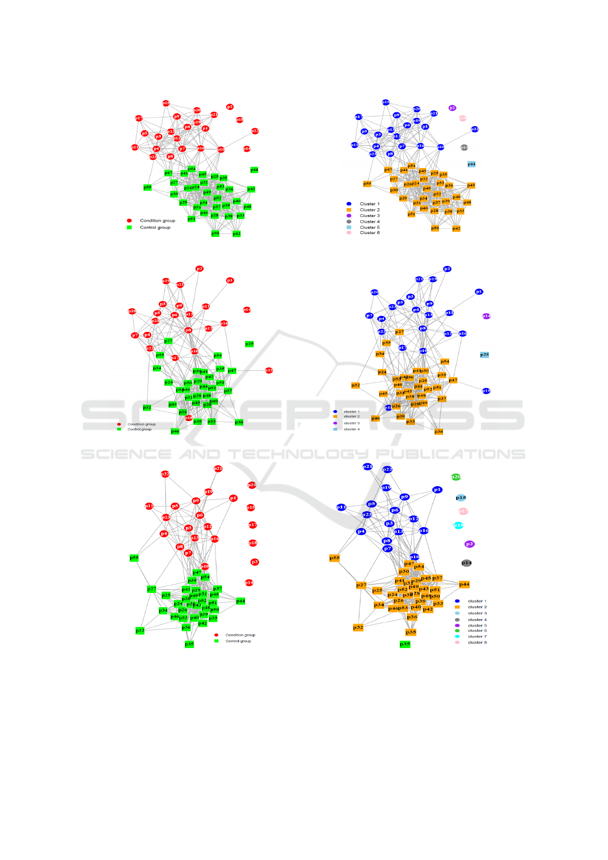
(a) M1:Correlation graph.

(b) M1:Clusters.

(e) M3:Correlation graph. (f) M3:Clusters.

Figure 2: Correlation graphs and discovered clusters.

The Comparison of Various Correlation Network Models in Studying Mobility Data for the Analysis of Depression Episodes

205

38 features, and the hybrid model (M3) has 86 fea-

tures. The Pearson correlation coefﬁcient is applied to

three models then M1 outputs 55x48 matrix, M2 out-

puts 55x38 matrix, and M3 yields 55x86 matrix. In

the next step, a predeﬁned threshold of 0.7, 0.6, and

0.55 are set to the models M1, M2, and M3 respec-

tively, to get the signiﬁcance matrix. A correlation

graph is generated from the three signiﬁcance matri-

ces. The obtained correlation graphs of M1, M2, and

M3 models are shown in Figure 2 (a, c, e). To rec-

ognize each person a unique id is used where con-

trol subjects are numbered from 1 to 23 and condition

groups are numbered from 24-55. Furthermore, con-

trol group participants are colored in green whereas

condition group subjects are colored in red. Each ver-

tex in the resultant correlation network represents an

individual while the edge between two vertices signi-

ﬁes the degree of similarity in terms of their move-

ment pattern.

Unraveling hidden clusters in a correlation graph

is a crucial step at this stage. MCL algorithm is

utilized to discover the potential clusters from three

graphs as depicted in Figure 2 (b, d, f). In this

graph, nodes with similar colors signify that they be-

long to the same community. we can comprehend

from the graph that controls and condition subjects

are fairly separated into two dense communities (con-

dition group in red color and control group is in green

color). Analyzing these communities provides nu-

merous insights into the connections between the in-

dividuals. Section 5 further elaborates on commonal-

ities between the persons in the same community.

5 DISCUSSION

In this section, a post hoc analysis is carried out on

the results obtained from the three models. The input

dataset consisting of mobility data collected from 55

subjects also provides classiﬁcation labels that corre-

spond to the diagnosis of the person. It is known from

the dataset that participants numbered from 1 to 23

belong to the condition group and they are diagnosed

with either unipolar or bipolar depression, whereas

subjects numbered from 24 to 55 belong to the healthy

control group. Previous studies that employed ma-

chine learning techniques had obtained higher ac-

curacy in terms of predicting the persons with and

without disorder (Garcia-Ceja et al., 2018) (Zanella-

Calzada et al., 2019) (Rodr

ıguez-Ruiz et al., 2020).

However, our hypothesis is not established based on

known labels rather we built the network by taking

advantage of the motor activity data itself. Therefore,

subgroups extracted from the correlation model are

more intuitive in terms of their movement patterns.

The main objective behind creating three models

is to understand the granularity of the mobility that

can best describe the overall movement patterns of

the subjects under study. From Figure 2, results ob-

tained from hour-wise mobility data are more promis-

ing than the other two models built on day-wise and

hybrid mobility data. Comparing three models shown

in Figure 2, M1 and M3 produced 6 clusters and M2

produced 4 clusters. However, all three models have

two dense clusters, and they mostly differ with respect

to the number of singleton or dual node clusters that

are not connected to the network. Model M1 has 6

clusters in which persons P2, P14, P18, and P44 are

isolated from the group. The phenomenon of isola-

tion highlights the peculiarity of these persons. They

are isolated because their mobility is not comparable

with any other person in the group. Nonetheless, from

the available information in the dataset, it is not possi-

ble to determine the exact reason behind their separa-

tion. Hence, we believe that having additional infor-

mation such as clinical parameters might be helpful

in further analysis. Additionally, the hourly features

employed for the M1 model separated condition and

control groups into two well-separated subgroups ac-

cording to their mobility but without using known la-

bels. Even though the M3 model divided condition

and control groups, P15 who is supposed to belong

to the condition group is clustered into the control

group. Similarly, in the M2 communities’ graph, P15

and P18 are classiﬁed as condition groups but they are

strongly correlated to control subjects than condition

subjects. By utilizing these rich insights, it is plau-

sible to comprehend the severity of the disorder pro-

vided if there is additional clinical information such

as medical history.

Another aspect of constructing three different

models is to realize the best method that can distin-

guish the subgroups according to the degree of mo-

bility. The creators of the dataset did not mention the

actual setting of the subjects under study. If all the

subjects are residing in the same community and have

the same daily routine, then day-wise segmentation

of the mobility data is helpful than the hourly seg-

mentation. Conversely, if the participants are living

in different communities with diverse daily routines,

then hourly features might produce better results than

day-wise features.

6 CONCLUSION

Mobility is considered one of the important inﬂuen-

tial factors that determine the overall health of an in-

BIOSIGNALS 2022 - 15th International Conference on Bio-inspired Systems and Signal Processing

206

dividual. However, certain medical conditions such

as depression can impact the mobility pattern. Conse-

quently, the affected individual’s movements are sig-

niﬁcantly altered compared to their healthy counter-

parts. However, the degradation in mobility can be

used as a vital parameter in characterizing the disor-

der. In the past, physicians assessed the depression

by an observation followed by self-reported feedback

from the patients. Yet, with the latest innovations in

wearable devices, it is possible to diagnose the ill-

ness by collecting mobility data from depressed pa-

tients using wearable sensors. In this study, we pro-

posed and built a correlation network model by utiliz-

ing the movement data collected from the group con-

sisting of depressed as well as healthy subjects. Ear-

lier studies predominantly focused on prediction of

the depression by incorporating known labels. How-

ever, our hypothesis is built on the concept of pop-

ulation analysis and correlation network by utilizing

the mobility data. We treated all the subjects belong-

ing to one group then explored similarities and differ-

ences between each pair of subjects by utilizing their

movement data. Then we constructed a correlation

network model that has the potential to discover the

subgroups of those who are suffering from depression

and healthy subjects. We have extracted three differ-

ent granularity of features and we found that hour-

wise features are the best set of feature parameters

that can fairly identify the subgroups.

REFERENCES

Abuse, S. (2018). Mental health services administra-

tion.(2017). key substance use and mental health in-

dicators in the united states: Results from the 2016

national survey on drug use and health (hhs publica-

tion no. sma 17-5044, nsduh series h-52). rockville,

md: Center for behavioral health statistics and qual-

ity. Substance Abuse and Mental Health Services

Administration. Retrieved from https://www. samhsa.

gov/data.

Ali, N., Neagu, D., and Trundle, P. (2019). Evaluation of

k-nearest neighbour classiﬁer performance for hetero-

geneous data sets. SN Applied Sciences, 1(12):1–15.

Curtin, S. C., Warner, M., and Hedegaard, H. (2016). In-

crease in suicide in the United States, 1999-2014.

Number 2016. US Department of Health and Human

Services, Centers for Disease Control and . . . .

Dongen, S. (2000). Performance criteria for graph cluster-

ing and Markov cluster experiments. CWI (Centre for

Mathematics and Computer Science).

Galv

an-Tejada, C. E., Zanella-Calzada, L. A., Gamboa-

Rosales, H., Galv

an-Tejada, J. I., Ch

avez-Lamas,

N. M., Gracia-Cort

es, M., Magallanes-Quintanar, R.,

Celaya-Padilla, J. M., et al. (2019). Depression

episodes detection in unipolar and bipolar patients: A

methodology with feature extraction and feature se-

lection with genetic algorithms using activity motion

signal as information source. Mobile Information Sys-

tems, 2019.

Garcia-Ceja, E., Riegler, M., Jakobsen, P., Tørresen, J.,

Nordgreen, T., Oedegaard, K. J., and Fasmer, O. B.

(2018). Depresjon: a motor activity database of de-

pression episodes in unipolar and bipolar patients. In

Proceedings of the 9th ACM multimedia systems con-

ference, pages 472–477.

Girvan, M. and Newman, M. E. (2002). Community struc-

ture in social and biological networks. Proceedings of

the national academy of sciences, 99(12):7821–7826.

Heinze, F., Hesels, K., Breitbach-Faller, N., Schmitz-Rode,

T., and Disselhorst-Klug, C. (2010). Movement anal-

ysis by accelerometry of newborns and infants for the

early detection of movement disorders due to infantile

cerebral palsy. Medical & biological engineering &

computing, 48(8):765–772.

Montgomery, S. A. and

Asberg, M. (1979). A new depres-

sion scale designed to be sensitive to change. The

British journal of psychiatry, 134(4):382–389.

Radloff, L. S. (1977). The ces-d scale: A self-report de-

pression scale for research in the general population.

Applied psychological measurement, 1(3):385–401.

Rodr

ıguez-Ruiz, J. G., Galv

an-Tejada, C. E., Zanella-

Calzada, L. A., Celaya-Padilla, J. M., Galv

an-

Tejada, J. I., Gamboa-Rosales, H., Luna-Garc

ıa, H.,

Magallanes-Quintanar, R., and Soto-Murillo, M. A.

(2020). Comparison of night, day and 24 h motor ac-

tivity data for the classiﬁcation of depressive episodes.

Diagnostics, 10(3):162.

Sobin, C. and Sackeim, H. A. (1997). Psychomotor symp-

toms of depression. American Journal of Psychiatry,

154(1):4–17.

The National Institute of Mental Health (NIMH) (2021).

Depression. [Online; accessed 8-August-2021].

The World Health Organization(WHO) (2021). Depression.

[Online; accessed 6-October-2021].

Zanella-Calzada, L. A., Galv

an-Tejada, C. E., Ch

avez-

Lamas, N. M., Gracia-Cort

es, M., Magallanes-

Quintanar, R., Celaya-Padilla, J. M., Galv

an-Tejada,

J. I., and Gamboa-Rosales, H. (2019). Feature extrac-

tion in motor activity signal: Towards a depression

episodes detection in unipolar and bipolar patients.

Diagnostics, 9(1):8.

The Comparison of Various Correlation Network Models in Studying Mobility Data for the Analysis of Depression Episodes

207