Modeling of Energy Consumption for Wired Access Control Systems

M. Oussayran

1,2

, J.-C. Pr

evotet

, J.-Y. Baudais

and A. Maiga

FDI MATELEC, Cholet, France

Univ. Rennes, INSA Rennes, CNRS, IETR-UMR 6164, F-35000 Rennes, France

Keywords:

Energy Consumption, Energy Model, Polling Protocol, Access Control System, Simulation Model, Wired

Network, OMNeT++.

Abstract:

Access control systems consist in managing access to buildings or any secure area where access is restricted.

This paper presents a model that helps build access control systems along with its internal architecture. This

system is modeled according to the behavior of the access control system. The OMNeT++ network simulator,

in addition to the INET framework, is used to model the behavior of a studied system as well as its energy

consumption. The paper aims to compare the energy consumption of the studied system and its simulated

model with the same working scenario. The challenge is to create a simulation model with a set of conﬁgurable

parameters, where users will be able to modify the value of the latter, based on the intended application. By this

way, the simulated model calculates promptly the energy consumption.

1 INTRODUCTION

Based on the published results on the energy consump-

tion in France (Minist

ere de la transition

ecologique,

2018), the two major consumers sectors are transport

and buildings, followed by the industry sector. Re-

garding the building sector, for new buildings and

major refurbishments, improvements in energy efﬁ-

ciency stemming from increasingly strict greenhouse

gas emissions targets is leading to a focus on techno-

logical improvements (Escriv

a-Escriv

a et al., 2010;

Moriarty and Honnery, 2019). The buildings sector is

divided into two sub-sectors: Residential and tertiary

sectors. In 2018, the residential sector in France hits

36 % of the total energy consumption, where 28 %

refers to the energy consumption of the home automa-

tion. A home automation system monitors and controls

home attributes such as lighting, climate, entertain-

ment systems, and appliances. It may also include

home security such as access control and alarm sys-

tems. Since 2019, the home automation market and

especially the smart security was worth US$ 21.8 bil-

lion, and expected to reach US$ 64.4 billion by the

year 2030 (Lee, 2021). Obviously, in case of increas-

ing the demand on the home security systems, the total

energy consumption of smart security systems will

also increase dramatically over the years.

Simply deﬁned, the term Access Control System

(ACS) describes any technique used to control pas-

sage into or out of any area. The standard lock that

uses a brass key may be thought of as a simple form

of an ACS. Over the years, ACSs have become pro-

gressively sophisticated, where different technologies

have widely emerged to improve usability and secu-

rity. Today, this term most often refers to a complex

computer-based or card-based access control system.

The electronic card access control system uses a spe-

cial access card or tag, rather than a brass key, to permit

access into the secured area (Domb, 2019). This sys-

tem is one of the home automation applications, where

its energy consumption might also be considered.

All these systems are ubiquitous in buildings and

becoming more and more complex. They often require

an associated management system that can also be very

sophisticated and power consuming. In this context, it

becomes very important to be able to optimize the per-

formance of such systems while reducing their power

consumption.

This paper highlights a simulation model of the

ACS is implemented in the OMNeT++ network simu-

lator with the addition of the INET 4.1.2 framework.

Using this framework, we are able to integrate several

functionalities such as the evaluation of the energy

consumption of each electronic component embedded

in the nodes. Also, it provides many MAC protocols

such as CSMA (Sanabria-Russo et al., 2013), SCM-

MAC (Ullah et al., 2013) etc., and makes it possible to

evaluate the performance of a given network and the

energy consumption in particular.

Over the decades, the energy consumption in net-

works has been studied widely (Bouguera et al., 2018).

144

Oussayran, M., Prévotet, J., Baudais, J. and Maiga, A.

Modeling of Energy Consumption for Wired Access Control Systems.

DOI: 10.5220/0010841300003118

In Proceedings of the 11th International Conference on Sensor Networks (SENSORNETS 2022), pages 144-151

ISBN: 978-989-758-551-7; ISSN: 2184-4380

 2022 by SCITEPRESS – Science and Technology Publications, Lda. All rights reser ved

Recently, many simulations models take into account

the sending, and the receiving activities to estimate

the energy consumption of the system. As well as,

the computation of the hardware components is ex-

tensively considered. Depending on the message rate

and the used duty-cycle, idle listening and message

reception can be even more costly than sending mes-

sages (Lebreton and Murad, 2015) (Le et al., 2013).

That why, we need to consider the communication as

well the computation energy consumption, in order to

estimate the global energy consumption of a system.

These models are developed based on the be-

haviour of real ACS modules and the energy models

are obtained using reference measures of real ACS. Af-

ter simulating the real scenario, we validate the ACS

model of the system by comparing results to those

obtained on a real ACS.

This paper is organized as follows. In Section 2,

we give a brief description of the ACS that is devel-

oped in OMNeT++. Section 3 presents the developed

ACS with its internal architecture including the mod-

eling of energy consumption. Simulations are listed

and discussed in Section 4. Finally, conclusions and

perspectives are given in Section 5.

2 ACS DESCRIPTION

The architecture of the studied ACS as well as the

communication between nodes are described in the

following parts.

2.1 Architecture

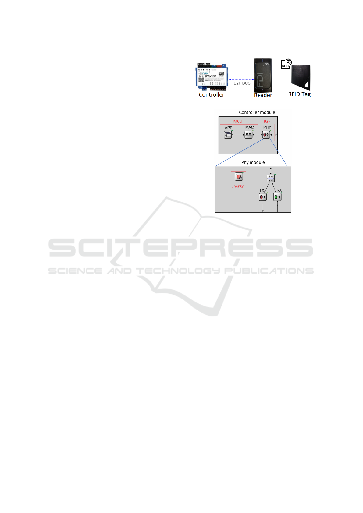
Figure 1 illustrates the architecture of the studied ACS.

This system consists of two interconnected nodes, the

controller node (CN) and the reader node (RN). The

RFID (Radio Frequency Identiﬁcation) tag is an end

user device used in the ACS. The communication be-

tween the RN and the CN is a wired connection, while

the communication between the end user RFID tag and

the RN is based on RFID technology. Once the RN

detects a tag in the proximity of its antenna, it reads

the tag’s data which they are related to the identity

of the end-user, then it sends a response to the CN.

Afterwards, the latter node will be charged to accept

or refuse the access request.

Nowadays, the ACS has become more and more so-

phisticated by integrating audio and video applications

as well as the radio communication (Barsocchi et al.,

2018) . Such system has emerged several technology

like RFID, Bluetooth, and so on, in order to provide

the multi-solutions provided in one system. Figure 2

shows the internal architecture of both nodes, where

Figure 1: Access control system architecture.

Figure 2: Model of ACS in OMNeT++.

only the main modules are illustrated. Other modules

like RS485, memory, BLE are not considered in the

scope of this paper, where those modules provide op-

tional solutions. The only module considered in this

paper are described as follow.

The Microcontroller.

The Microcontroller (MCU)

manages all the resources utilized for the system oper-

ation. This block is responsible for acquiring output

data, processing data after acquisition, generating new

data and communicate the new generated data to the

B2F circuit.

The B2F Circuit.

The B2F circuit has been invented

by the same company who developed the studied ACS.

This circuit couples power and data on a single wire,

which is also considered as a communication bus.

Through this bus, the reader and the controller nodes

are connected where they communicate according to

the speciﬁed communication protocol. Therefore, the

circuit takes in charge the transmission and the recep-

tion of data packets. We should note that the electronic

circuits, related to the B2F implemented in the CN and

the RN, are completely different.

The RFID Module.

The RFID system consists of

a tiny radio transponder, a radio receiver and a trans-

mitter. Through these units, an RFID module is able

to detect a proximity tag near its antenna. The RFID

Modeling of Energy Consumption for Wired Access Control Systems

145

Figure 3: Polling access control method: (a) Without tag; (b)

With tag.

module is implemented in the RN whereas the tag also

implements a passive RFID system.

2.2 Communication between Nodes

The communication between nodes is based on the

polling protocol, in which master and slave architec-

tures must be selected. In the studied ACS, the CN

is the master node, whereas the RN is the slave node.

Using polling as a controlled access protocol for net-

works, the communication is managed by the master.

The RN then communicates only when it receives a

request from the CN.

The ACS presents a limitation with its connection

capabilities where only one RN is able to be connected

to the CN. In case, we connect more than one RN to

the CN, the communication will not establish due the

the frequent collision occurred on the bus. Figure 3 (a)

and 3 (b) depicts, respectively, the communication

sequences in absence and presence of the end user

RFID tag close to the RN’s antenna.

The polling protocol is as follow. Initially, the CN

requests, by sending a poll request, the RN to verify

if there is any RFID tag close to the RN’s antenna.

After that, the RN veriﬁes through its RFID module

and then responds to the CN. In case where the RN

has not detected an RFID tag, the RN sends a packet

accordingly. Hence, a new polling request will be sent

after a predeﬁned delay. This delay is one on the main

parameters to be integrated in the ACS model. In the

other case, where the reader detect a RFID tag, the

RN responds to the CN, then the CN requests more

information about the detected tag. At the end of

the second case, the CN acknowledges the RN. This

communication sequence refers to the actual scenario

implemented in the studied ACS. The time spent to

read an RFID is difﬁcult to be estimated accurately,

because this time depends on many factors, mainly the

types of the tag, the antenna, etc. .

In the following, we introduce the system model-

ing, where the studied ACS has been modeled includ-

ing the described protocols.

3 SYSTEM MODELING IN

OMNeT++

Based on several surveys and research (Patel et al.,

2018), (Kabir et al., 2014), OMNeT++ has been cho-

sen to model the global system. This simulator is a

widely used network simulator by both academic and

research communities. The last ten years have shown

that the OMNeT++ approach is viable, and several

OMNeT++ based open-source simulation models and

model frameworks have been published by various re-

search groups and individuals (Birajdar and Solapure,

2017). One of the main motivations of using OM-

NeT++ is to model the communication channel and

the associated polling protocol, by taking advantage

of the features provided by the INET framework.

In the previous section, we mentioned the main

components used in the ACS. To enable prediction of

the energy consumption, we must take into account a

detailed model of the components embedded in con-

troller and reader nodes. The ﬁrst challenge for the

prediction of the energy consumption is to build a de-

tailed energy model of the ACS. Our approach for

such a model consists of three steps: (1) We measured

the current consumption of each state of all the ACS

internal modules while running a speciﬁc application;

(2) The model derived from these measurements, for

example, the power consumption of the modules states,

is implemented in the ACS model; (3) The model must

be calibrated and simulated according to the measured

ACS.

3.1 Experimental Setup

An application has been developed and deployed on

the ACS. During the program execution, we are able

to measure the current draw of various combinations

of modules states using a digital multimeter. Figure 4

depicts the methods used to measure the current of

each internal module. The MCU module operates as a

Finite State Machine (FSM), where each state executes

a speciﬁc task. Also, the B2F circuit operates based an

its own developed FSM. Those FSM will be discussed

in details later. The multi-meter measures the current

consumption at the input of each module. Furthermore,

the time spent in each operating state is also estimated.

Figure 5 illustrates the measured current of the RN’s

B2F circuit, using the DMM7510 multi-meter. Based

on the developed application, we determined the be-

SENSORNETS 2022 - 11th International Conference on Sensor Networks

146

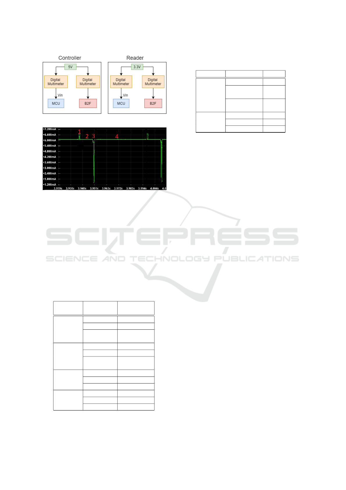
Figure 4: Current measurements of the ACS.

Figure 5: The measured current consumption of the RN’s

B2F circuit.

havior of the circuit. Four successive sequences are

mentioned in the latter ﬁgure. Each sequence is de-

ﬁned by an operating state. We extracted the draw of

current of each module’s state and calculated its power

consumption.

Finally, the estimated power consumption of each

module forms our intended energy model for the ACS.

As the ACS is mainly based on electronic components,

potential results might deviate from the power con-

sumption measurements. Table 1 compiles the values

employed to characterize the nodes used in the ACS.

Table 1: Power consumption of the nodes’ modules.

Devices States Power

consumption

CN MCU

Idle 26 mW

Transmit 32 mW

Receive

and Process

28 mW

RN MCU

Idle 28 mW

Transmit 31 mW

Receive

and Process

31 mW

CN B2F

Idle 44 mW

Transmit 10 mW

Receive 49 mW

RN B2F

Idle 20 mW

Transmit 5 mW

Receive 22 mW

Table 2: Main characteristics of the communication cycle

without tag.

Devices States Time

CN MCU

Idle 48 ms

Generate

and Transmit

0.9 ms

Receive

and Process

1.1 ms

CN B2F

Idle 48 ms

Transmit 0.9 ms

Receive 0.9 ms

Table 2 shows the time spent during the commu-

nication sequence without a tag. The MCUs embed-

ded in both nodes are running with the same clock

frequency. Moreover, the polling request and the re-

sponse have both the same packet length (4 bytes).

Therefore, the generation time and the transmission

time required by the RN’s MCU is identical to the

CN’s MCU. Finally, the idle time spent in the CN’s

MCU is also the same and similar to the idle time of

the B2F circuits.

3.2 Nodes Modeling

Both CN and the RN contain many internals elec-

tronic components such as RFID, BLE, accelerometer,

RS485, Wiegand, etc. . Considering the modeling of

these components, it potentially increases the complex-

ity of the implementation and the simulation time can

be slower than expected. That is why, we decided to

abstract their behavior while guaranteeing a high level

of accuracy when dealing with power consumption.

The implemented design is outlined in Figure 2. In

this work, we look toward modeling the system as a

network, where nodes communicate with respect to

the polling protocol.

Both nodes of the ACS are modeled with their in-

ternal modules, where these modules are implemented

according to their layers. For example, the MCUs

are modeled according to two layers: Application and

MAC, whereas the B2F circuit is modeled according

to its PHY layer. The RFID device, embedded in the

RN, is also modeled as an application layer. The B2F

circuits are modeled as a transmitter and a receiver

modules in both nodes. Figure 6 depicts the mod-

ules’ layers implemented in the reader and the con-

troller nodes. Each modules takes into account only

the power consumption of its internal layer. Therefore,

the power consumption of the RN’s MCU does not

include the consumed power of the RN’s RFID appli-

cation layer. In this paper, we mainly focused on the

energy consumption of the MCUs and B2F circuits.

Modeling of Energy Consumption for Wired Access Control Systems

147

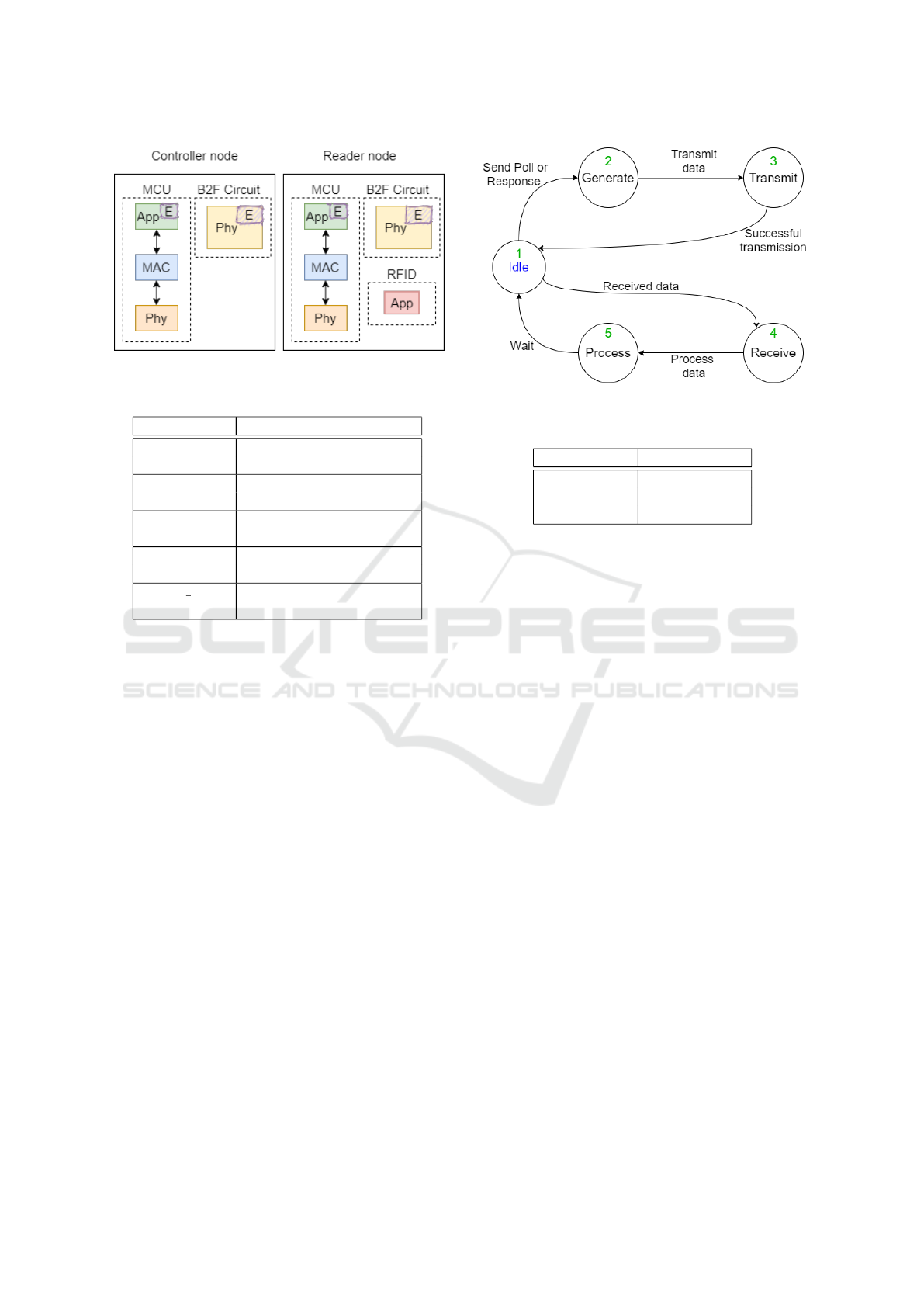
Figure 6: Layers modeling for ACS’ nodes.

Table 3: Model parameters.

Parameters Explanations

iaTime Inter arrival time between

two detected tags (s)

PacketLength Different packet length

to be assigned (Byte)

Bitrate Communication speed

(actual speed: 38400 kbps)

NbRN Number of connected

reader nodes

MCU Freq Operating frequency of

the MCU (MHz)

MCU States.

To identify the operating state of the

MCU and precisely its application layer during the

operation, we modeled the application layer as a FSM.

This makes it possible to integrate the intended commu-

nication by adding several adjustable parameters. For

example, a given parameter may be related to the time

duration required to process a data packet. Other pa-

rameters are integrated, such as data rate, packet length

etc., where most of them are adjustable to simulate dif-

ferent nodes’ conﬁgurations. Table 3 lists some of the

integrated parameters. Leveraging of these parameters,

the energy consumption of the intended application

could be promptly estimated.

Figure 7 illustrates the operating states of the MCU

and its transition sequences for both nodes. Initially,

the MCU is in the idle state. After a predeﬁned delay,

the controller’s MCU switches from its idle state to

the generate state in order to generate the appropri-

ate polling packet. After the generation time which

depends on the running frequency of the MCU, this

latter transmits the generated packet then returns back

to the idle state. The controller MCU receives and

then processes the data packets sent by the reader. The

described states’ transition are related to the controller

MCU, where this sequence is periodically performed.

The following sequence refers to the operating states

Figure 7: The operating states of the MCUs.

Table 4: States of B2F circuit.

Working state Transition state

Idle Idle to transmit

Transmit Idle to receive

Receive

occurred by the RN’s MCU: 1, 4, 5, 1, 2, 3 (see Fig-

ure 7) and then, the MCU returns back to the idle state,

waiting for a new request from the CN.

B2F States.

Regarding the B2F circuit, the operating

states are listed in Table 4, as well as the correspond-

ing states’ transition. The B2F circuit is responsible

for transmitting and receiving data accordingly. All

these states are implemented according to the applica-

tion requirements. Based on these states, the energy

consumption has been evaluated.

Note that the B2F circuit is made by off-the-shelf

electronic components (e.g. resistances, transistors).

This circuit has been developed to perform communi-

cation through two wires, where power and data are

coupled on the same wire. This circuit has some lim-

itation and drawback, where the maximum bitrate is

38400 bps and the power consumption during the idle

state is higher than the transmitting state. This power

consumption literally depends on the behavior of the

circuits.

3.3 Energy Modeling

After modeling the nodes on OMMeT++, we take

advantage of the INET framework to integrate the

power consumption for each element embedded in the

nodes. In this framework, several existing features

were commonly used to model the energy of the ACS.

The energy model computes the energy consumption

of the modules based on the power that is speciﬁed

during operating states.

SENSORNETS 2022 - 11th International Conference on Sensor Networks

148

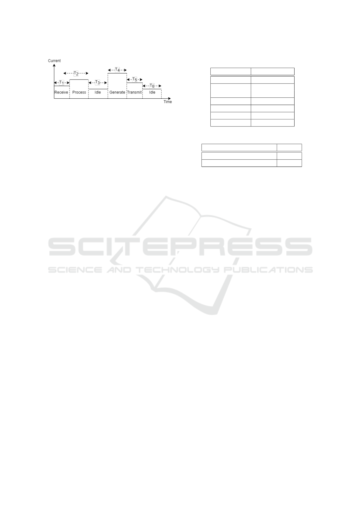
Figure 8: State-based energy consumption modeling.

Since most implemented layers are modeled as

FSM, in which each operating state of a module is

described, we are able to assign a power consumption

value to each of these states. Each module has its own

energy model, where the energy models of the MCUs

are implemented in the MCU’s application layer, and

the energy models of the B2F circuits is modeled in

the B2F circuit’s PHY layer.

Typically, using simulators, the energy consump-

tion is modeled by rather simple state-based ap-

proaches, where the time

of the module, i.e., the

MCU or the B2F circuit, being in a state

is recorded

and multiplied with the maximum current

in state

as well as the constant supply voltage

to calculate

the energy consumption. We further have to sum up

the energy consumed

by the duration

in each state.

Equation 1 determines

, the overall consumed energy

by a module.

E =

∑

i=1

· I

· U (1)

where N expresses the number of operating states for

a module.

Figure 8 illustrates the working sequence of the

MCU module used in both nodes. This module is

in on-state all along the working sequence because it

manages the different operating modes.

During the measurement phase of the ACS, the

power consumption of the ACS tends to ﬂuctuate in

each operating state. As the power consumption in

the operating states is not stable, the maximum mea-

sured power consumption is considered. In that way,

the integrated power in the energy model refers to the

maximum power measured with the ACS. The energy

consumed to generate a packet, transmit it through its

pins, receive a packet, etc. is tracked by the energy

model. Models are able to calculate energy consump-

tion during a predeﬁned simulation time.

We faced some difﬁculties while measuring the

power consumption during the communication cycle

when RN ’s has a tag. In this case, The estimated time

and power were complicated to be estimated correctly

due to fast ﬂuctuations. Thereby, the energy model

during this communication cycle is not integrated ad-

equately. Thus, the energy model of the CN’s B2F

circuit may deviate.

Table 5: Model parameters of the ACS application scenario.

Parameters Values

iaTime 40 ms

PacketLength polling request

(4 Byte)

Bitrate 38400 kbps

NbRN 1

NbCN 1

Freq. MCU 64 MHz

Table 6: Simulation time of the modeled ACS.

Case Time

Communication without tag 50 ms

Communication with tag 400 ms

4 SIMULATIONS AND

DISCUSSIONS

In this section, we study the modeled system by simu-

lating the same scenario as the actual ACS. The imple-

mented scenario has been described in Section 2.2.

4.1 Network Simulation

To illustrate the simulation model of the ACS, the con-

sidered application has been developed to compare the

energy consumption of the measured ACS against the

simulated model. Table 5 lists some of the parame-

ters that are calibrated in order to run the simulation

similarly to the measured ACS.

Two communication sequences were integrated in

the simulation model. We ran two different simula-

tions, one is related to the communication sequence

without a tag, the other refers to the communication

sequence along with a tag detected. For each simula-

tion, we were able to measure the energy consumption

during one operating cycle, except for the CN’s B2F

circuit, which was really complex because of the cur-

rent ﬂuctuations. The operating cycle specify the time

between requesting two successive polling request.

Table 6 lists the operating cycle time. While the com-

munication without tag, we estimated that the period

between to successive request is approximately 50 ms.

For the communication sequence with tag detected,

the time depends on many parameters related to the

end user tag and the component’s tolerance embedded

in the RN. Nonetheless, we estimated its period by

attempting several tests using the ACS.

Modeling of Energy Consumption for Wired Access Control Systems

149

4.2 Simulation Results

In this section, we present the energy consumption

measured as well as simulation using the developed

energy model. Validating is important for reliable and

accurate results. We discussed about the energy mea-

sured using the digital current measurements equip-

ment and the estimated current integrated into the en-

ergy models.

Energy Consumption of the Simulated ACS.

The

following table 7 lists the energy consumption of the

modules while the RN has not detected tags. The mea-

sured energy consumption is calculated by the equa-

tion 2, where the average current has been calculated

with the ACS.

E = I

avg

· U · T (2)

Where

avg

is the average current measured, and

the time of one operating cycle.

With both equations (1, 2), the voltage

is as-

signed with the adequate value. For example, the MCU

of the CN is powered with 4.8 V, meanwhile the MCU

module embedded in the RN is powered by 3.2 V. The

difference between the measured and the simulated

energy consumption depends mainly on the current

consumption. The error between the simulated and

the measured energy consumption is determined by

the equation 3. This error presents the deviation be-

tween the average current measured and the maximum

current integrated in the energy models.

AbsoluteError(%) =

− E

× 100 (3)

The measured value of the CN’s MCU is approxi-

mately 1.3 mJ, whereas the simulated value is 1.4 mJ.

The main difference in those value is due to current

consumption that ﬂuctuates during operating states,

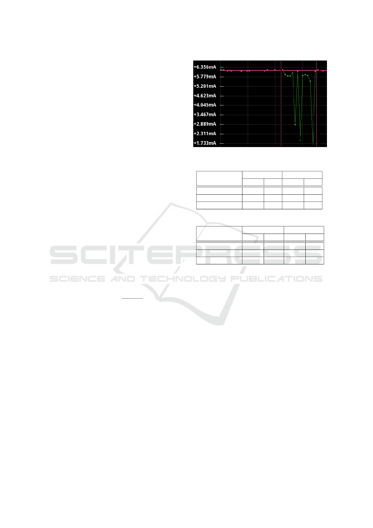
except in the idle state. An example of the current ﬂuc-

tuation is depicted in Figure9. A packet of response

polling is transmitted to the CN B2F circuit.

The difference between the measured energy con-

sumption and the simulated is less than 5

. We mod-

eled this system with the aim to validate the simulated

ACS along with its energy model. It must be noted

that it is not possible to simulate precisely the behavior

of MCU and B2F circuit compared to their real-time

operations, especially during detecting a tag. This ab-

solute error value is regarded as acceptable given the

lack of power measurement precision. We note that

the power consumption integrated in the energy model

is stable during the operating states. Meanwhile, in

measured ACS, the power consumption oscillates in

uncontrollable behavior.

Figure 9: Current consumption of the transmitting state.

Table 7: Energy consumption without detected tag.

No tags

CN RN

MCU B2F MCU B2F

Measured (mJ) 1.3 7.5 1.4 1.02

Simulated (mJ) 1.4 7.8 1.36 1.03

Error (%) 1.3 3.8 2.8 0.9

Table 8: Energy consumption with detected tag.

Tag detected

CN RN

MCU B2F MCU B2F

Measured (mJ) 115 671k 90.9 64.3

Simulated (mJ) 107 587k 93.02 63.3

Error (%) 6.9 12.5 2.2 1.4

Table 8 lists the energy consumption of the mod-

ules while the RN detects a tag. When RN’s detect

a tag, the measurement was not sufﬁciently accurate.

Therefore, a deviation of 12.5 % for the CN’s B2F

circuit is observed due to these limitations.

Synthesis.

During the ﬁrst communication sequence,

when the RN has not detected a tag, the communica-

tion was implemented precisely due to its simplicity.

The energy model calculates the energy consumption

based on the current draw for each operating state.

Some parameters related to the operating states has

been reconﬁgured in order to analyze the feasibility of

the energy model with different application scenarios.

We ﬁnd that the energy model behaves as expected.

For example, when the parameter iaTime is assigned a

value of 80 ms, we noted that the energy consumption

decreases.

Regarding the second communication sequence

related to a tag detected by the RN, the difference be-

tween the measured and the simulated energy is due to

the complexity of the communication sequence, espe-

cially for the CN’s B2F circuit. We have modeled the

B2F circuit as a PHY layer working with three operat-

ing states. As the measured and the simulated energy

SENSORNETS 2022 - 11th International Conference on Sensor Networks

150

consumption are very close, we validated the energy

model implemented in OMNeT++. However, we can

use this modeling for future studies with the aim to

reduce the global energy consumption effectively.

5 CONCLUSION AND FUTURE

WORK

In this paper, we presented the access control system

used to limit the physical access to any secured and

restricted area. The architecture and the internal mod-

ules of the ACS are presented in details. This work

focuses on the energy consumption of the communi-

cation and the computation of hardware devices used

in the studied systems. A simulation environment for

ACS based on OMNeT++ and the INET framework is

described as well. The purpose of this paper is to com-

pare the energy consumption of the studied system and

its simulated model with the same working scenario.

After the implementation and the calibration phases,

both energies were calculated to evaluate the system’s

performance, where we have validated the modeled

system. For future works, we will study and simulate

several conﬁgurations in order to achieve better energy

efﬁciency. We will also take into account their impacts

on the ACS quality of service (QoS). In addition, we

argue that evaluating the energy performance with a

single RN is not enough to assess the network. There-

fore, we will evaluate different scenarios dealing with

multiple interconnected systems.

REFERENCES

Barsocchi, P., Calabr

o, A., Ferro, E., Gennaro, C., Marchetti,

E., and Vairo, C. (2018). Boosting a low-cost smart

home environment with usage and access control rules.

Sensors, 18(6).

Birajdar, D. M. and Solapure, S. S. (2017). Leach: An energy

efﬁcient routing protocol using omnet++ for wireless

sensor network. In International Conference on Inven-

tive Communication and Computational Technologies

(ICICCT), pages 465–470.

Bouguera, T., Diouris, J.-F., Chaillout, J.-J., and Andrieux,

G. (2018). Energy consumption modeling for com-

municating sensors using LoRa technology. In IEEE

Conference on Antenna Measurements and Applica-

tions, CAMA, page Paper No.1029, V

aster

as, Sweden.

Domb, M. (2019). Smart Home Systems Based on Internet

of Things. Proceedings of the 10th INDIACom; 3rd In-

ternational Conference on Computing for Sustainable

Global Development, INDIACom, pages 2073–2075.

Escriv

a-Escriv

a, G., Segura-Heras, I., and Alc

azar-Ortega,

M. (2010). Application of an energy management and

control system to assess the potential of different con-

trol strategies in hvac systems. Energy and Buildings,

42(11):2258–2267.

Kabir, M., Islam, S., Hossain, M., and Hossain, S. (2014).

Detail comparison of network simulators. Interna-

tional Journal of Scientiﬁc and Engineering Research,

5(10):203–218.

Le, T.-N., Magno, M., Pegatoquet, A., Berder, O., Sentieys,

O., and Popovici, E. (2013). Ultra Low Power Asyn-

chronous MAC Protocol using Wake-Up Radio for

Energy Neutral Wireless Sensor Networks. In Interna-

tional Workshop on Energy-Neutral Sensing Systems,

pages 1–6, Rome, Italy.

Lebreton, J.-M. and Murad, N. (2015). Implementation

of a Wake-up Radio Cross-Layer Protocol in OM-

NeT++/MiXiM. In OMNeT++ Community Summit,

pages 1–5, Zurich, Switzerland.

Lee, G. (2021). Smart homes: Inside a new fast growing

market, set to be worth $75bn by 2025. Naval Technol-

ogy.

Minist

ere de la transition

ecologique (2018). French strategy

for energy and climate. Executive summary.

Moriarty, P. and Honnery, D. (2019). Energy efﬁciency or

conservation for mitigating climate change? Energies,

12(18):1–17.

Patel, R. L., Pathak, M. J., and Nayak, A. J. (2018). Sur-

vey on network simulators. International Journal of

Computer Applications, 182(21):23–30.

Sanabria-Russo, L., Faridi, A., Bellalta, B., Barcelo, J., and

Oliver, M. (2013). Future evolution of csma protocols

for the ieee 802.11 standard. In International Confer-

ence on Communications, pages 1274–1279, Budapest,

Hungary.

Ullah, A., Ahn, J.-S., and Kim, G. (2013). X-mac protocol

with collision avoidance algorithm. In International

Conference on Ubiquitous and Future Networks, pages

228–233, Da Nang, Vietnam.

Modeling of Energy Consumption for Wired Access Control Systems

151