
Subclass-based Undersampling for Class-imbalanced Image
Classification
Daniel Lehmann and Marc Ebner
Institut f
¨
ur Mathematik und Informatik, Universit
¨
at Greifswald
Walther-Rathenau-Straße 47, 17489 Greifswald, Germany
Keywords:
Undersampling, Clustering, CNN.
Abstract:
Image classification problems are often class-imbalanced in practice. Such a class imbalance can negatively
affect the classification performance of CNN models. A State-of-the-Art (SOTA) approach to address this issue
is to randomly undersample the majority class. However, random undersampling can result in an information
loss because the randomly selected samples may not come from all distinct groups of samples of the class
(subclasses). In this paper, we examine an alternative undersampling approach. Our method undersamples
a class by selecting samples from all subclasses of the class. To identify the subclasses, we investigated if
clustering of the high-level features of CNN models is a suitable approach. We conducted experiments on 2
real-world datasets. Their results show that our approach can outperform a) models trained on the imbalanced
dataset and b) models trained using several SOTA methods addressing the class imbalance.
1 INTRODUCTION
Image classification datasets are often imbalanced in
practice. Certain classes contain significantly less
frequent samples (minority classes) than the other
classes (majority classes). A dataset of images show-
ing healthy plants and plants suffering from a plant
disease, for instance, will be imbalanced if the plant
disease occurs rarely in nature (minority class: plant
with disease, majority class: healthy plant). A Con-
volutional Neural Network (CNN) model trained on
this dataset may not perform well for images of the
less frequent class. During training, the mini-batches
mostly contain images of the majority class as they
occur more frequently in the data. Hence, the result-
ing model may only have learned a proper representa-
tion of the majority class but not of the minority class.
A State-of-the-Art (SOTA) approach to address
this problem is random undersampling (Buda et al.,
2018; Lee et al., 2016; More, 2016). Random un-
dersampling balances a dataset by randomly select-
ing samples of the majority class until the number
of picked majority class samples is approximately as
high as the number of minority class samples. Then, a
model is trained using the minority class samples and
the selected majority class samples. A disadvantage
of this approach, however, is that it can lose infor-
mation about the majority class. A class may con-
tain different groups of images (Nguyen et al., 2016;
Wei et al., 2015) (subclasses). The ImageNet (Rus-
sakovsky et al., 2015) class baseball, for instance, can
be grouped into images showing a baseball player
and images showing only the ball. If samples from
the baseball class are randomly selected, then the se-
lected samples may come mostly from only one of the
2 subclasses. As a consequence, a model trained on
such an undersampled dataset will not have learned
a proper representation of the baseball class as it has
not seen enough samples from both subclasses.
In this work, we examine an alternative approach
to undersample the majority class. Our method se-
lects samples from every subclass. Before we can
select any samples, however, we must first find the
subclasses within the majority class samples. To iden-
tify the subclasses, we use clustering on the high-level
features of the CNN model. Using this undersam-
pling method, we state 2 research questions: 1) Is
clustering of the high-level image features of a CNN
model beneficial for undersampling, and 2) is our ap-
proach able to outperform a model trained on the im-
balanced dataset as well as models using SOTA meth-
ods addressing the class imbalance? Our experiments
show that both questions can be answered with yes.
Our contributions are as follows: 1) We show that
clustering of the high-level image features of a CNN
model is beneficial for undersampling, 2) we pro-
Lehmann, D. and Ebner, M.
Subclass-based Undersampling for Class-imbalanced Image Classification.
DOI: 10.5220/0010841100003124
In Proceedings of the 17th International Joint Conference on Computer Vision, Imaging and Computer Graphics Theory and Applications (VISIGRAPP 2022) - Volume 5: VISAPP, pages
493-500
ISBN: 978-989-758-555-5; ISSN: 2184-4321
Copyright
c
2022 by SCITEPRESS – Science and Technology Publications, Lda. All rights reserved
493

pose a subclass-based undersampling approach that
selects the majority class samples more carefully than
a random undersampling, and 3) we show (on 2 real-
world datasets) that our method can outperform sev-
eral SOTA methods addressing the class imbalance.
2 RELATED WORK
To improve random undersampling, various methods
have been suggested. Kubat and Matwin (Kubat and
Matwin, 1997) introduced one-sided selection, which
identifies redundant samples close to a class bound-
ary. Zhang and Mani (Zhang and Mani, 2003) pro-
posed a method that selects samples according to the
distance between the majority and minority class sam-
ples. Garcia and Herrera (Garc
´
ıa and Herrera, 2009)
suggested an evolutionary undersampling. Majumder
et. al. (Majumder et al., 2020) proposed a method
based on feature vector angles to pick the samples that
contain the most information. Koziarski (Koziarski,
2020a) introduced a radial-based undersampling. Liu
et. al. (Liu et al., 2009) proposed EasyEnsemble
and BalanceCascade. EasyEnsemble is an ensemble
method that picks different subsets of the majority
class and trains a model for each of them. Balance-
Cascade, in contrast, trains a model sequentially. In
each iteration, the correctly classified majority class
samples are removed from the training set. However,
the methods most similar to ours are cluster-based
(Agrawal et al., 2015; Sowah et al., 2016; Tsai et al.,
2019; Yen and Lee, 2009) and hashing-based under-
sampling (Ng et al., 2020). Cluster-based undersam-
pling attempts to find clusters in the dataset and then
selects samples from each identified cluster. Hashing-
based undersampling, in contrast, uses hashing to di-
vide the majority class into subspaces. However, both
methods have been suggested for tabular data and can
not be used for image data directly. Our method, in
contrast, is applied to images used for CNN training.
We investigated if clustering of high-level image fea-
tures can be used for undersampling.
Besides undersampling, several other approaches
have been proposed to address model training using
a class-imbalanced dataset. A widely used approach
is oversampling, which creates additional samples for
the minority class to balance the dataset. A sim-
ple method to oversample a class is to duplicate ran-
domly selected samples of that class (More, 2016).
Singh and Dhall (Singh and Dhall, 2018) improved
this method by not selecting samples randomly for
duplication but based on the distance of a sample to
its cluster centroid. Besides duplicating samples, var-
ious methods have been suggested to oversample a
minority class by creating synthetic samples for that
class (Ando and Huang, 2017; Chawla et al., 2002;
Hao et al., 2020; Mullick et al., 2019). Shen et.
al. (Shen et al., 2016) do not create any samples
but uniformly populate the mini-batches with sam-
ples from all classes during model training. Kozarski
(Koziarski, 2020b) introduced a method that com-
bines oversampling and undersampling. Furthermore,
there has been work that addresses the class im-
balance by introducing a special loss function (Cao
et al., 2019; Dong et al., 2017; More, 2016; Sarkar
et al., 2020), a balanced group softmax (Li et al.,
2020), dynamic sampling (Pouyanfar et al., 2018),
dynamic curriculum learning (Wang et al., 2019),
cost-sensitive learning (Khan et al., 2015), a local
embedding (Huang et al., 2016) or category centers
(Zhang et al., 2018). Category centers are also used
in high-level image feature space. However, the cen-
ters are exploited for the classification process and not
to undersample the dataset as our method does.
3 METHOD
Our undersampling method can be applied to multi-
class imbalanced image datasets containing several
majority classes. To balance such a dataset, our
method must be applied to each majority class sep-
arately. Thus, in order to explain our method, we
consider a two-class imbalanced dataset containing
only one majority class in the following without los-
ing generality. We undersample the majority class in
2 stages. First, we identify the subclasses of the ma-
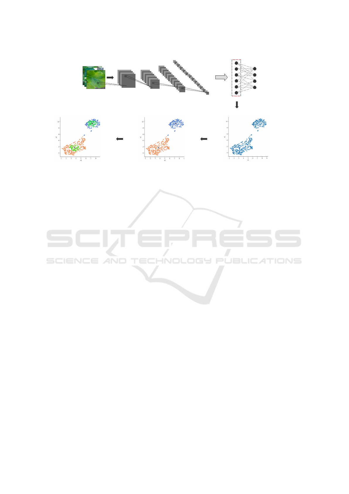
jority class (as shown in steps 1 to 4 in Figure 1). Sec-
ond, we select representative samples from each iden-
tified subclass (as shown in step 5 in Figure 1). The
selected majority class samples and all minority class
samples form the new undersampled dataset. We de-
scribe both stages in more detail below.
In order to identify subclasses of the majority
class C, we use a method similar to that suggested
by Nguyen et. al. (Nguyen et al., 2016). However,
Nguyen et. al. introduced their method to visualize
multifaceted features learned by a CNN. We adapted
their method to find representative samples of a class
for undersampling that class. First, we train an ini-
tial model f
0
using the imbalanced training set (X, Y).
The resulting model f
0
may not perform well for the
minority class as it is underrepresented in the data.
We assume, however, the model f
0
learns at least a
sufficient representation of the majority class C. After
we trained the model f
0
, we use this model to extract
features from each image x
C
of the majority class C.
We assume C has N
C
samples x
C
in the training set
VISAPP 2022 - 17th International Conference on Computer Vision Theory and Applications
494
2) Choose Layer
Pool
1) Feed Images of
and Reduce to 2D
3) Fetch Activations
5) Select
Samples
4) Clustering
the Class to CNN
Figure 1: Our method: 1) Feed majority class images into the initial CNN model (trained on the imbalanced dataset), 2)
choose a layer from which to fetch activations, 3) fetch activations of the images at the chosen layer and reduce activations to
2D, 4) find clusters in the activations and 5) select samples from each identified cluster.
(X, Y ). In order to extract the features, we feed all N
C
images x
C
into model f
0
. At a certain layer L, we fetch
the layer activations of each image x
C
. The activations
represent the features that layer L extracts from the
images x
C
. Which layer to pick depends on the classi-
fication problem to solve. It is important, however, to
choose one of the last layers of the CNN (i.e., closer
to the output layer). The last layers of a CNN extract
high-level features (e.g., object parts), while the ear-
lier layers extract low-level features (e.g., edges, sim-
ple shapes) as shown by Zeiler and Fergus (Zeiler and
Fergus, 2014). In order to identify subclasses repre-
senting different semantic concepts (e.g., the subclass
baseball player and the subclass ball from the Ima-
geNet class baseball), we must use the high-level fea-
tures from one of the last network layers as only these
features are characteristic for the different semantic
concepts. If the chosen layer is a convolutional layer,
the fetched activations of each image x
C
will be in
cube form. To convert the activations to vector form,
we flatten the activations. If the chosen layer is a lin-
ear layer, however, the fetched activations will be in
vector form already, and we do not need to flatten
them. In either case, we receive N
C
feature vectors
a
x
C
(one from each image x
C
) of length M
L
. Then, we
concatenate all N
C
vectors a
x
C
to a feature matrix A
C
of size N
C
× M
L
.
In the data of the matrix A
C
, we try to find clus-
ters representing different subclasses of C. Before we
can apply clustering on the data, however, we need to
reduce the dimensions of the feature matrix A
C
from
N
C
× M
L
down to N
C
× 2. This preprocessing step is
necessary as clustering is usually more difficult to ap-
ply in high dimensions (Chen et al., 2019). First, we
normalize A
C
by subtracting the mean and then di-
viding by the standard deviation (prerequisite for di-
mensionality reduction). Then, we project A
C
from
N
C
×M
L
down to N
C
×50 using PCA (Pearson, 1901)
followed by a second reduction from N
C
×50 down to
N
C
× 2 using UMAP (McInnes et al., 2018). As a re-
sult, we receive the projected features matrix p(A
C
)
of size N
C
× 2. The reason why we use PCA and
UMAP combined is that A
C
is usually too large to
directly apply a non-linear dimensionality reduction
technique such as UMAP. On the other hand, using
only a linear dimensionality reduction (such as PCA)
did not result in a sufficient data representation in our
experiments. Thus, we use a combination of both
techniques. A similar approach was also suggested
by Ngyuen et. al. (Nguyen et al., 2016). Finally,
we apply k-Means clustering (MacQueen, 1967) on
p(A
C
) to identify clusters in the feature data. To find
the parameter k, we apply k-Means multiple times us-
ing different k (values: 2-9) and compute the Silhou-
ette score (Rousseeuw, 1987) of the resulting clusters
for each k. The Silhouette score is an evaluation met-
ric that measures the cluster quality using the mean
inter-cluster and mean intra-cluster distance (range:
between -1 and 1, a higher score means a better cluster
quality). As Chen et. al. (Chen et al., 2019) pointed
out, this score works well for evaluating clusters in
the layer activations of a CNN. Thus, we choose the k
that obtained the best Silhouette score. As a result, we
receive 1, ..., k clusters, which represent the potential
subclasses of the majority class.
After identifying 1, ..., k clusters in p(A
C
), we se-
lect a certain number of representative samples x
C
u
k
from each cluster 1, ..., k. For instance, if we need
to select 100 majority class samples, and we found 2
clusters, we will select 50 samples from each identi-
Subclass-based Undersampling for Class-imbalanced Image Classification
495

fied cluster. In order to select the samples from each
cluster, we consider 2 options: a) We select the sam-
ples from each cluster that are closest to their cluster
center, and b) we select the samples from each cluster
that are farthest from their cluster center (excluding
outliers). The most representative samples of a clus-
ter should be samples closest to their cluster center.
Therefore, we chose to examine option a). On the
other hand, however, the samples closest to a cluster
center may be quite similar if these samples are close
to each other as well. We would like to select samples
that are as unique as possible when undersampling the
data. Thus, we also examine option b) by selecting
the samples of a cluster that are most far away from
their cluster center. In order to avoid selecting out-
liers (e.g., noise, mislabeled samples), however, we
only consider the 80th percentile of all the samples of
a cluster. After selecting the samples x
C
u
k
from each
cluster 1, ..., k using one of the 2 options, we merge
these samples together with all minority class sam-
ples to obtain the undersampled dataset (X
u
, Y
u
). This
dataset can be used to train a new model f
u
.
4 EXPERIMENTS
4.1 Experimental Setup
We conducted several experiments to test our method
described in section 3. For each experiment, we
executed the following steps: 1) Training an initial
model, 2) selecting a layer of that model, 3) feeding
all training images of the class that should be under-
sampled to the model and fetching their activations at
the selected layer, 4) finding clusters in the fetched
activations, 5) picking a certain number of samples
from each cluster, 6) using the picked samples and
all training images from the other classes that should
not be undersampled as the new training set, 7) train-
ing a model using the new undersampled training set,
and 8) comparing this model to a model trained on
the imbalanced training set (baseline) and to models
trained using SOTA methods addressing the class im-
balance (e.g., through random undersampling, over-
sampling, a class-weighted loss) with respect to their
performance on the test set.
For our experiments we used the datasets from 2
image classification competitions hosted on the data
science platform Kaggle: a) The Plant Pathology
2020
1
competition (Thapa et al., 2020) and b) the
1
https://www.kaggle.com/c/plant-pathology-2020-
fgvc7
Fisheries Monitoring
2
competition. The Plant Pathol-
ogy dataset has 4 classes. One of the classes con-
tains significantly fewer images than the other classes.
The Fisheries Monitoring dataset, in contrast, has 8
classes. One of the classes contains significantly more
images than the other classes.
We used the same training setup for all of our
models. Except for our experiments in section 4.4,
we chose a ResNet50 (He et al., 2016) as model ar-
chitecture. All models were pretrained on ImageNet
(Russakovsky et al., 2015). We removed the output
layer (for the ImageNet classes) and replaced it with
the following new layers: A combination of an adap-
tive average pooling layer and an adaptive max pool-
ing layer (output of both are concatenated) - Batch-
Norm - Dropout (p = 0.25) - Linear layer (size: 512)
- ReLU - BatchNorm - Dropout (p = 0.5) - Linear out-
put layer. Each model was fine-tuned using a discrim-
inative fine-tuning strategy (Howard and Ruder, 2018)
in a two-stage process. First, we fine-tuned only the
initial weights of the new layers (which we added)
for 3 epochs. Then, we fine-tuned the weights of all
layers of the network for 8 more epochs. The learning
rate was set to an initial value of 0.01 and was then ad-
justed over the course of training via a cyclical learn-
ing rate schedule (Smith, 2017). We used mixed pre-
cision training (Micikevicius et al., 2018) to be able to
set the batch size to 25. For the Plant Pathology data,
we adopted all data augmentation techniques from
the original winner
3
of the corresponding competition
(brightness, contrast, blur, shift, scale, rotation, hori-
zontal and vertical flip). For the Fisheries Monitoring
data, we used the same data augmentation techniques
except for the vertical flip. Unlike the Plant Pathol-
ogy images, the images of the Fisheries Monitoring
dataset were always taken from the same vertical ori-
entation. All images of both datasets were resized to
224 × 224 before training.
Each model was evaluated using the Kaggle sub-
mission system. The submission system evaluates the
Plant Pathology competition using the ROC AUC
1
metric, while it evaluates the Fisheries Monitoring
competition using the multi-class logarithmic loss
2
(LogLoss). Kaggle splits the test set of a competition
into 2 parts: A public and a private test set. While
the competition is active, the submission system only
shows how a model performed on the public test set.
When the competition is over, the evaluation score on
the private test set will be visible as well. The user
with the best score on the private test set wins the
competition. As the Plant Pathology and the Fish-
2
https://www.kaggle.com/c/the-nature-conservancy-
fisheries-monitoring
3
https://github.com/alipay/cvpr2020-plant-pathology
VISAPP 2022 - 17th International Conference on Computer Vision Theory and Applications
496
Table 1: Comparison of our method (selecting closest/farthest samples to cluster center) to the baseline (imbalanced dataset)
and random undersampling on the Plant Pathology data. All models were trained over 6 random seeds. The results are
reported as median ROC AUC scores (a higher value is better) and standard deviations (std) over the 6 seeds.
Method Undersampled Class ROC AUC
median std
Baseline - 0.9387 0.0045
Random Undersampling healthy 0.9375 0.0086
rust 0.9187 0.0092
scab 0.9377 0.0024
healthy, rust, scab 0.9068 0.0233
Ours (closest) healthy 0.9391 0.0058
rust 0.9171 0.0069
scab 0.9425 0.0088
healthy, rust, scab 0.8909 0.0166
Ours (farthest) healthy 0.9353 0.0059
rust 0.9183 0.0098
scab 0.9369 0.0080
healthy, rust, scab 0.9004 0.0054
eries Monitoring competition are both not active any-
more, the evaluation scores on the private test set are
already available for both competitions. Thus, we use
the scores on the private test set to evaluate our mod-
els as these are crucial for winning the competitions.
4.2 Selecting Closest Samples
We conducted an experiment to test whether our un-
dersampling approach using the closest samples to
each identified cluster center (as described in section
3) is able to improve model performance. As the Plant
Pathology dataset contains 3 majority classes (rust,
scab and healthy), we examined 4 different under-
sampling strategies: 1) Undersampling of the healthy
class only (from 516 to 100 samples), 2) undersam-
pling of the rust class only (from 622 to 100 samples),
3) undersampling of the scab class only (from 592 to
100 samples) and, 4) undersampling of the healthy,
rust and scab class (to 100 samples per class). To be
able to find clusters in the data of a majority class,
our method requires choosing a layer whose activa-
tions should be used for clustering. We considered
the last 3 layers before the output layer of the network.
Among these 3 layers, we chose the layer whose ac-
tivations reached the best Silhouette score. For rust
and healthy, we obtained the best Silhouette score us-
ing the activations of the adaptive pooling layer (con-
catenation of average and max pooling), while for
scab the last linear layer before the output layer re-
sulted in the best Silhouette score. For each class, we
picked the same number of samples from each iden-
tified cluster. For instance, we found 2 clusters in the
data of the healthy class. Therefore, we picked 50
samples closest to each cluster center to obtain 100
samples in total for that class. As a result, we re-
ceived the following datasets: a) One undersampled
dataset from our method for each strategy 1) - 4), b)
the baseline (imbalanced dataset) and c) 6 randomly
undersampled datasets (More, 2016) (using a differ-
ent random seed each time for the random sampling)
for each strategy 1) - 4). With each of these datasets,
we trained 6 models using a different random seed
each time and report the median test performance over
the 6 models. The results are shown in Table 1.
The Fisheries Monitoring dataset contains 1 ma-
jority class (ALB class). As a result, we undersampled
only this class (from 1719 to 734 samples). Again, we
selected the same number of samples from each iden-
tified cluster. We obtained the best Silhouette score
using the activations of the last ResNet50 layer before
the newly added layers. Thus, we used these layer ac-
tivations to undersample the class. Then, we trained a
model (1 seed) using a) the dataset undersampled by
our method (using the closest samples), b) the base-
line (imbalanced dataset), and c) 5 randomly under-
sampled datasets (More, 2016) (using a different ran-
dom seed each time for the random sampling). The
results of our experiment for the Fisheries Monitor-
ing data are shown in Table 2.
4.3 Selecting Farthest Samples
In another experiment, we tested if our undersam-
pling approach using the farthest samples from each
identified cluster center is able to improve model per-
formance. The experimental setup was the same as
in section 4.2, except for the method how to pick
the samples. Instead of selecting the closest samples
to each cluster center, we undersampled the data by
Subclass-based Undersampling for Class-imbalanced Image Classification
497
Table 2: Comparison of our method to the baseline (imbal-
anced dataset) and random undersampling (median over 5
random samplings) on the Fisheries Monitoring data (un-
dersampling of class ALB). The results are reported as
multi-class logarithmic loss (a lower value is better).
Method LogLoss
Baseline 5.7333
Random Undersampling 4.0771
Ours (closest) 3.8657
Ours (farthest) 3.9302
picking the farthest samples from each cluster center,
as described in section 3. The results of the experi-
ment for the Plant Pathology data are shown in Table
1, and the results of the experiment for the Fisheries
Monitoring data are shown in Table 2. In contrast to
section 4.2, however, we obtained the best Silhouette
score for the Fisheries Monitoring dataset using the
activations of the adaptive pooling layer. Thus, we
used these layer activations for undersampling.
4.4 Other CNN Architectures
In our experiments in section 4.2 and section 4.3, we
used a pretrained ResNet50 for all our models, as de-
scribed in section 4.1. To examine how our under-
sampling approach performs using other CNN archi-
tectures, we conducted additional experiments for the
healthy class (516 samples) of the Plant Pathology
data. The experimental setup was the same as for the
experiments in section 4.2 and section 4.3, except for
the CNN architecture. We examined 2 additional ar-
chitectures: a) DenseNet121 (Huang et al., 2017) and
b) VGG16 (Simonyan and Zisserman, 2015) (with
BatchNorm (Ioffe and Szegedy, 2015)). A model
was trained (1 seed) for each architecture using a)
the dataset undersampled by our method (to 100 sam-
ples), b) the baseline (imbalanced dataset), and c)
5 randomly undersampled datasets (More, 2016) (to
100 samples using a different random seed each time
for the random sampling). The results of the experi-
ment are shown in Table 3.
4.5 Comparison to SOTA Methods
In our experiments in section 4.2, 4.3 and 4.4 we only
compared our method to the baseline (imbalanced
dataset) and random undersampling (More, 2016). In
another experiment, we examined how our method
performs in comparison to other SOTA methods ad-
dressing data imbalance applied to the Plant Pathol-
ogy dataset: a) oversampling (More, 2016) of the
minority class (multiple diseases class, 91 samples)
and b) a training approach using a class-weighted loss
function (More, 2016). For oversampling, we tested 2
Table 3: Comparison of our method to the baseline (imbal-
anced dataset) and random undersampling (median over 5
random samplings) with respect to different CNN architec-
tures on the Plant Pathology data (undersampling of class
healthy). The results are reported as ROC AUC scores (a
higher value is better).
Method CNN Arch. ROC AUC
Baseline VGG16 0.9435
Rand. Undersamp. 0.9404
Ours (closest) 0.9447
Ours (farthest) 0.9322
Baseline DenseNet121 0.9461
Rand. Undersamp. 0.9384
Ours (closest) 0.9294
Ours (farthest) 0.9465
approaches: 1) duplicating the minority class samples
2 times (resulting in 182 samples), and b) duplicating
the minority class samples 6 times (resulting in 546
samples). For the class-weighted loss function, we set
the weights for each class according to the fraction
of samples of that class among the total number of
samples of the Plant Pathology dataset. Moreover, we
tested 2 additional configurations for undersampling
the healthy class using our method. First, besides se-
lecting the closest samples to each cluster center and
selecting the farthest samples from each cluster cen-
ter, we also selected samples from each cluster ran-
domly. Second, besides undersampling the healthy
class from 516 to 100 samples, we also undersampled
the healthy class from 516 to 250 samples. We trained
a model (1 seed) for each method. The results of the
experiment are shown in Table 4.
Table 4: Comparison of our method (undersampling of class
healthy) to the baseline (imbalanced dataset), random un-
dersampling, oversampling, and a class-weighted loss ap-
proach on the Plant Pathology data. The results are reported
as ROC AUC scores (a higher value is better).
Method ROC AUC
Baseline 0.9343
Class-Weighted Loss 0.9466
Oversampling (182 samples) 0.9469
Oversampling (546 samples) 0.9268
Rand. Undersamp. (100 samples) 0.9370
Ours (closest, 100 samples) 0.9451
Ours (farthest, 100 samples) 0.9301
Ours (random, 100 samples) 0.9377
Rand. Undersamp. (250 samples) 0.9474
Ours (closest, 250 samples) 0.9488
Ours (farthest, 250 samples) 0.9453
Ours (random, 250 samples) 0.9551
VISAPP 2022 - 17th International Conference on Computer Vision Theory and Applications
498

5 CONCLUSION
In section 1, we stated 2 research questions: 1) Is
clustering of the high-level image features of a CNN
model beneficial for undersampling, and 2) is our
approach able to outperform a model trained on the
imbalanced dataset as well as models using SOTA
methods addressing the class imbalance? Our ex-
periments (section 4) show that our method is able
to obtain a better performance than the baseline and
a random undersampling. Moreover, our method is
also able to surpass the performance of other SOTA
methods addressing data imbalance (oversampling,
class-weighted loss). Selecting the closest samples
to each cluster center for undersampling the majority
class performed best in most cases in our experiments.
However, there were also cases in which selecting the
farthest samples from each cluster center or a ran-
dom cluster sample selection reached a better perfor-
mance. As a result, we have shown that a subclass-
based undersampling is able to surpass the perfor-
mance of a model trained on the imbalanced dataset
(baseline) and models trained using SOTA methods
addressing the class imbalance. This could also be
helpful for other research areas. In medical imag-
ing, for instance, datasets are frequently imbalanced
as well (Larrazabal et al., 2020; Reza and Ma, 2018).
Furthermore, datasets in practice often contain label
noise (Algan and Ulusoy, 2021; Xiao et al., 2015),
i.e., some images of a dataset were inadvertently mis-
labeled. In future work, it could be investigated if we
can identify such noise using our method.
REFERENCES
Agrawal, A., Viktor, H. L., and Paquet, E. (2015).
Scut: Multi-class imbalanced data classification using
smote and cluster-based undersampling. In IC3K, vol-
ume 1, pages 226–234, Lisbon, Portugal. IEEE.
Algan, G. and Ulusoy, I. (2021). Image classification with
deep learning in the presence of noisy labels: A sur-
vey. Knowledge-Based Systems, 215:106771.
Ando, S. and Huang, C. Y. (2017). Deep over-sampling
framework for classifying imbalanced data. In Ceci,
M., Dzeroski, S., Vens, C., Todorovski, L., and Holl-
men, J., editors, ECML PKDD, Lecture Notes in CS,
pages 770–785. Springer.
Buda, M., Maki, A., and Mazurowski, M. A. (2018). A
systematic study of the class imbalance problem in
convolutional neural networks. Neural Networks,
106:249–259.
Cao, K., Wei, C., Gaidon, A., Arechiga, N., and Ma, T.
(2019). Learning imbalanced datasets with label-
distribution-aware margin loss. In Wallach, H.,
Larochelle, H., Beygelzimer, A., d'Alch
´
e-Buc, F.,
Fox, E., and Garnett, R., editors, Adv Neural Inf Pro-
cess Syst, volume 32, Vancouver, CA. CAI.
Chawla, N. V., Bowyer, K. W., Hall, L. O., and Kegelmeyer,
W. P. (2002). Smote: Synthetic minority over-
sampling technique. Journal of Artif Int Res,
16(1):321–357.
Chen, B., Carvalho, W., Baracaldo, N., Ludwig, H., Ed-
wards, B., Lee, T., Molloy, I., and Srivastava, B.
(2019). Detecting backdoor attacks on deep neu-
ral networks by activation clustering. In Espinoza,
H., h
´
Eigeartaigh, S.
´
O., Huang, X., Hern
´
andez-
Orallo, J., and Castillo-Effen, M., editors, Workshop
on SafeAI@AAAI, volume 2301 of CEUR Workshop,
Honolulu, HI, USA. ceur-ws.org.
Dong, Q., Gong, S., and Zhu, X. (2017). Class rectification
hard mining for imbalanced deep learning. In ICCV,
pages 1869–1878, Venice, Italy. IEEE.
Garc
´
ıa, S. and Herrera, F. (2009). Evolutionary undersam-
pling for classification with imbalanced datasets: Pro-
posals and taxonomy. Evol Comput, 17(3):275–306.
Hao, J., Wang, C., Zhang, H., and Yang, G. (2020). An-
nealing genetic gan for minority oversampling. ArXiv,
abs/2008.01967.
He, K., Zhang, X., Ren, S., and Sun, J. (2016). Deep resid-
ual learning for image recognition. In CVPR, pages
770–778, Las Vegas, NV, USA. IEEE.
Howard, J. and Ruder, S. (2018). Universal language model
fine-tuning for text classification. In Proc of the ACL,
pages 328–339, Melbourne, Australia. ACL.
Huang, C., Li, Y., Loy, C. C., and Tang, X. (2016). Learning
deep representation for imbalanced classification. In
CVPR, pages 5375–5384, Las Vegas, NV, USA. IEEE.
Huang, G., Liu, Z., Van Der Maaten, L., and Weinberger,
K. Q. (2017). Densely connected convolutional net-
works. In CVPR, pages 2261–2269, Honolulu, HI,
USA. IEEE.
Ioffe, S. and Szegedy, C. (2015). Batch normalization:
Accelerating deep network training by reducing in-
ternal covariate shift. In Bach, F. and Blei, D., edi-
tors, ICML, volume 37 of Proc Mach Learn Res, page
448–456, Lille, France. PMLR.
Khan, S. H., Hayat, M., Bennamoun, M., Sohel, F., and
Togneri, R. (2015). Cost sensitive learning of deep
feature representations from imbalanced data. ArXiv,
abs/1508.03422.
Koziarski, M. (2020a). Radial-based undersampling for
imbalanced data classification. Pattern Recognition,
102:107262.
Koziarski, M. (2020b). Two-stage resampling for con-
volutional neural network training in the imbal-
anced colorectal cancer image classification. ArXiv,
abs/2004.03332.
Kubat, M. and Matwin, S. (1997). Addressing the curse
of imbalanced training sets: One-sided selection. In
ICML, pages 179–186. Morgan Kaufmann.
Larrazabal, A. J., Nieto, N., Peterson, V., Milone, D. H.,
and Ferrante, E. (2020). Gender imbalance in med-
ical imaging datasets produces biased classifiers for
computer-aided diagnosis. Proc National Academy of
Sciences, 117(23):12592–12594.
Subclass-based Undersampling for Class-imbalanced Image Classification
499

Lee, H., Park, M., and Kim, J. (2016). Plankton classifica-
tion on imbalanced large scale database via convolu-
tional neural networks with transfer learning. In ICIP,
pages 3713–3717, Phoenix, AZ, USA. IEEE.
Li, Y., Wang, T., Kang, B., Tang, S., Wang, C., Li, J., and
Feng, J. (2020). Overcoming classifier imbalance for
long-tail object detection with balanced group soft-
max. In CVPR, pages 10991–11000.
Liu, X.-Y., Wu, J., and Zhou, Z.-H. (2009). Exploratory
undersampling for class-imbalance learning. Trans.
Sys. Man Cyber. Part B, 39(2):539–550.
MacQueen, J. B. (1967). Some methods for classification
and analysis of multivariate observations. In Cam,
L. M. L. and Neyman, J., editors, Berkeley Symp on
Math Stat and Prob, volume 1, pages 281–297. Univ
of Calif Press.
Majumder, A., Dutta, S., Kumar, S., and Behera, L. (2020).
A method for handling multi-class imbalanced data
by geometry based information sampling and class
prioritized synthetic data generation (gicaps). ArXiv,
abs/2010.05155.
McInnes, L., Healy, J., and Melville, J. (2018). UMAP:
Uniform manifold approximation and projection for
dimension reduction. ArXiv, abs/1802.03426.
Micikevicius, P., Narang, S., Alben, J., Diamos, G., Elsen,
E., Garcia, D., Ginsburg, B., Houston, M., Kuchaiev,
O., Venkatesh, G., and Wu, H. (2018). Mixed preci-
sion training. In ICLR, Vancouver, CA.
More, A. (2016). Survey of resampling techniques for
improving classification performance in unbalanced
datasets. ArXiv, abs/1608.06048.
Mullick, S. S., Datta, S., and Das, S. (2019). Generative
adversarial minority oversampling. In ICCV, pages
1695–1704, Seoul, South Korea. IEEE.
Ng, W. W., Xu, S., Zhang, J., Tian, X., Rong, T., and
Kwong, S. (2020). Hashing-based undersampling
ensemble for imbalanced pattern classification prob-
lems. Transactions on Cybernetics.
Nguyen, A., Yosinski, J., and Clune, J. (2016). Multifaceted
feature visualization: Uncovering the different types
of features learned by each neuron in deep neural net-
works. ArXiv, abs/1602.03616.
Pearson, K. (1901). LIII. On lines and planes of closest
fit to systems of points in space. London, Edinburgh
Dublin Philos Mag J Sci, 2(11):559–572.
Pouyanfar, S., Tao, Y., Mohan, A., Tian, H., Kaseb, A. S.,
Gauen, K., Dailey, R., Aghajanzadeh, S., Lu, Y. H.,
Chen, S. C., and Shyu, M. L. (2018). Dynamic sam-
pling in convolutional neural networks for imbalanced
data classification. In MIPR, Proc MIPR 2018, pages
112–117. Inst Electrical and Electronics Engineers
Inc.
Reza, M. S. and Ma, J. (2018). Imbalanced histopatholog-
ical breast cancer image classification with convolu-
tional neural network. In ICSP, pages 619–624. IEEE.
Rousseeuw, P. J. (1987). Silhouettes: A graphical aid to
the interpretation and validation of cluster analysis. J.
Comput. Appl. Math., 20(1):53–65.
Russakovsky, O., Deng, J., Su, H., Krause, J., Satheesh, S.,
Ma, S., Huang, Z., Karpathy, A., Khosla, A., Bern-
stein, M., Berg, A. C., and Fei-Fei, L. (2015). Ima-
genet large scale visual recognition challenge. IJCV,
115(3):211–252.
Sarkar, D., Narang, A., and Rai, S. (2020). Fed-focal loss
for imbalanced data classification in federated learn-
ing. ArXiv, abs/2011.06283.
Shen, L., Lin, Z., and Huang, Q. (2016). Relay backprop-
agation for effective learning of deep convolutional
neural networks. In Leibe, B., Matas, J., Sebe, N., and
Welling, M., editors, ECCV, volume 9911 of Lecture
Notes in CS, pages 467–482. Springer.
Simonyan, K. and Zisserman, A. (2015). Very deep convo-
lutional networks for large-scale image recognition. In
Bengio, Y. and LeCun, Y., editors, ICLR, San Diego,
CA, USA.
Singh, N. D. and Dhall, A. (2018). Clustering and learning
from imbalanced data. ArXiv, abs/1811.00972.
Smith, L. N. (2017). Cyclical learning rates for training
neural networks. In WACV, pages 464–472. IEEE.
Sowah, R. A., Agebure, M. A., Mills, G. A., Koumadi,
K. M., and Fiawoo, S. Y. (2016). New cluster under-
sampling technique for class imbalance learning. Int
Journal of Mach Learning and Computing, 6(3):205.
Thapa, R., Zhang, K., Snavely, N., Belongie, S., and Khan,
A. (2020). The plant pathology challenge 2020 data
set to classify foliar disease of apples. Appl in Plant
Sciences, 8(9):e11390.
Tsai, C.-F., Lin, W.-C., Hu, Y.-H., and Yao, G.-T. (2019).
Under-sampling class imbalanced datasets by combin-
ing clustering analysis and instance selection. Infor-
mation Sciences, 477:47–54.
Wang, Y., Gan, W., Yang, J., Wu, W., and Yan, J. (2019).
Dynamic curriculum learning for imbalanced data
classification. In ICCV, pages 5016–5025, Seoul,
South Korea. IEEE.
Wei, D., Zhou, B., Torrabla, A., and Freeman, W. (2015).
Understanding intra-class knowledge inside CNN.
ArXiv, abs/1507.02379.
Xiao, T., Xia, T., Yang, Y., Huang, C., and Wang, X. (2015).
Learning from massive noisy labeled data for image
classification. In CVPR, pages 2691–2699, Boston,
MA, USA. IEEE.
Yen, S.-J. and Lee, Y.-S. (2009). Cluster-based under-
sampling approaches for imbalanced data distribu-
tions. Expert Systems with Applications, 36(3):5718–
5727.
Zeiler, M. D. and Fergus, R. (2014). Visualizing and un-
derstanding convolutional networks. In Fleet, D., Pa-
jdla, T., Schiele, B., and Tuytelaars, T., editors, ECCV,
number PART 1 in Lecture Notes in CS, pages 818–
833, Zurich, CH. Springer.
Zhang, J. and Mani, I. (2003). kNN approach to unbalanced
data distributions: A case study involving information
extraction. In Proc ICML Workshop on Learning from
Imbalanced Datasets, volume 126.
Zhang, Y., Shuai, L., Ren, Y., and Chen, H. (2018). Image
classification with category centers in class imbalance
situation. In YAC, pages 359–363.
VISAPP 2022 - 17th International Conference on Computer Vision Theory and Applications
500
