A Step Towards Learning Contraction Kernels for Irregular Image
Pyramid
Darshan Batavia
1 a
, Rocio Gonzalez-Diaz
2 b
and Walter G. Kropatsch
1 c
1
TU Wien, Pattern Recognition and Image Processing Group 193/03, Vienna, Austria
2
University of Seville, Department of Applied Math I, Seville, Spain
Keywords:
Cost of Contraction Kernels, Dictionary for Contraction Kernel, Irregular Image Pyramid, Slope Region.
Abstract:
A structure preserving irregular image pyramid can be computed by applying basic graph operations (contrac-
tion and removal of edges) on the 4-adjacent neighbourhood graph of an image. In this paper, we derive an
objective function that classifies the edges as contractible or removable for building an irregular graph pyra-
mid. The objective function is based on the cost of the edges in the contraction kernel (sub-graph selected for
contraction) together with the size of the contraction kernel. Based on the objective function, we also provide
an algorithm that decomposes a 2D image into monotonically connected regions of the image surface, called
slope regions. We proved that the proposed algorithm results in a graph-based irregular image pyramid that
preserves the structure and the topology of the critical points (the local maxima, the local minima, and the
saddles). Later we introduce the concept of the dictionary for the connected components of the contraction
kernel, consisting of sub-graphs that can be combined together to form a set of contraction kernels. A favorable
contraction kernel can be selected that best satisfies the objective function. Lastly, we show the experimental
verification for the claims related to the objective function and the cost of the contraction kernel. The outcome
of this paper can be envisioned as a step towards learning the contraction kernel for the construction of an
irregular image pyramid.
1 INTRODUCTION
Graph-based representations are the primary object
of study for many pattern recognition and computer
vision application areas. Graphs are capable of rep-
resenting both structured and unstructured data as-
sociated with applications ranging from processing
2D images to social network analysis and climate
data analysis. Out of several approaches to encounter
graph-based processing, this paper focuses on the
construction of an irregular image pyramid computed
from a 2D image, such that the topology and the struc-
ture of the image are preserved blue in a concise man-
ner at the higher levels of the pyramid. The pro-
posed objective function is used to predict an opti-
mal contraction kernel that governs the construction
of an irregular image pyramid. In the broader con-
text, the proposed algorithm decomposes a 2D Eu-
clidean space into cells that are represented by critical
a
https://orcid.org/0000-0003-0062-3411
b
https://orcid.org/0000-0001-9937-0033
c
https://orcid.org/0000-0003-4915-4118
points (the local maximum, the local minimum, and
the saddle) and the connections between them. As
mentioned in (Helman and Hesselink, 1991), a com-
pact representation of a 2D image can be achieved by
using a surface topology-based data structure.
There is an extensive literature on similar ap-
proaches for the decomposition of the 2D spaces, es-
pecially for the decomposition of the Morse-Smale
complex (MS-complex). As mentioned in (Stein
et al., 1963), the Morse-Smale complex is a collec-
tion of the Morse cells that follow a smooth function
on a manifold, h : M 7→ R such that all the critical
points are non-degenerated. Nackman Lee in (Lee,
1984) represents a surface in form of graphs of crit-
ical points, subdividing the surface into slope dis-
tricts. Other approaches include: Reeb graph (Shina-
gawa et al., 1991), hierarchical decomposition of MS-
complex into piece-wise linear 2-manifolds (Edels-
brunner et al., 2003). Many efficient algorithms
can be found in the literature to compute consis-
tent MS complexes. For example, in (Gyulassy
et al., 2014), the authors presented an efficient al-
gorithm to compute consistent MS complexes using
60
Batavia, D., Gonzalez-Diaz, R. and Kropatsch, W.
A Step Towards Learning Contraction Kernels for Irregular Image Pyramid.
DOI: 10.5220/0010840900003122
In Proceedings of the 11th International Conference on Pattern Recognition Applications and Methods (ICPRAM 2022), pages 60-70
ISBN: 978-989-758-549-4; ISSN: 2184-4313
Copyright
c
 2022 by SCITEPRESS – Science and Technology Publications, Lda. All rights reserved

a divide-and-conquer strategy for dealing with large
data. In (Comic et al., 2010), the authors computed
maximal cells of the ascending and the descending
Morse complexes through a watershed approach.
In reality, 2D images may contain degenerated
critical points and thus they cannot be treated as MS-
complexes before any pre-processing. Therefore, in
this paper, we focus on a more generic framework
that allows the presence of degenerated critical points.
In (Gonzalez-Diaz et al., 2021), the authors explained
a hierarchical approach for the decomposition of any
surface into cells called slope regions and proved the
necessary and sufficient conditions for the existence
of the slope regions. The authors in (Batavia et al.,
2019) described the partitioning of an image into
slope regions. Utilizing these theories, in (Batavia
et al., 2020), the authors used the combinatorial pyra-
mid framework to build irregular image pyramids and
displayed results for over-segmented images and im-
age reconstruction from the top level of the graph
pyramid while preserving the texture information. A
similar framework were used by Morales-Gonzalez et
al. in (Morales-Gonz
´
alez and Garc
´
ıa-Reyes, 2013)
for the application of object recognition and object
matching.
The main goal of this paper is to express the al-
gorithm mentioned in (Batavia et al., 2020) for irreg-
ular image pyramid in form of an objective function
and introduce the dictionary for the connected com-
ponents of the contraction kernel. The paper is or-
ganized as follows: Section 2 introduces and defines
the basic terminology and the motivation behind this
work. Then, we derive the objective function and
explain the algorithm for building the irregular im-
age pyramid. In Section 4, we show a novel concept
of a dictionary for the connected components of the
contraction kernel, consisting of a generic set of sub-
graphs that can be used in combination to construct
a favorable contraction kernel. Experimental verifica-
tion and statistical evidences are shown in Section 5
for the claims made in Section 3. Then, we conclude
the paper with the conclusions and the future work.
2 DEFINITIONS AND
MOTIVATION
A 2D image P can be visually perceived as a sampled
version of a geographical terrain model in 2.5D with
a continuous height (intensity) map h : R
2
→ [0, 1].
A pixel p ∈ P is a discrete sample obtained by sam-
pling the 2.5D continuous surface. The digital im-
age P can be effectively represented by a planar 4-
connected neighbourhood graph G
0
= (V
0
, E
0
), where
every pixel p in the image P corresponds to a vertex
v ∈ V
0
with gray value g(v) := h(p) ∈ [0, 1].
With help of basic graph operations, namely the
edge contraction and the edge removal, we can reduce
the graph size. Stacking up the reduced graphs will
result in a formation of an irregular graph pyramid.
The k
th
level of an irregular graph pyramid is denoted
by G
k
(V
k
, E
k
) where V
k
and E
k
are the set of vertices
and edges respectively, and k ∈ {0, 1, . . . , n} outlines
the level of the graph pyramid. |E
k
| and |V
k
| denotes
the cardinality of the edge set E
k
and of the vertex set
V
k
, respectively.
For each edge (v, w) ∈ E
k
, where v, w ∈ V
k
,
there is an attribute contrast c(e) := |g(v) − g(w)|.
The edges are oriented from vertex v to vertex
w if g(v) > g(w), if g(v) = g(w) they are non-
oriented. A connected sub-graph of G
k
having
the same gray value for all the vertices is re-
ferred to as a plateau region (connected sub-graph
of degenerated vertices). A path π(v
1
, v
2
, . . . , v
r
) =
(V
π
, E
π
) is defined as a nonempty sub-graph of
G
k
(V
k
, E
k
), where V
π
= {v
1
, v
2
, . . . , v
r
} ⊆ V
k
and E
π
=
{(v
1
, v
2
), (v
2
, v
3
), . . . , (v
r−1
, v
r
)} ⊆ E
k
. The path π is
monotonic if all the oriented edges of E
π
have the
same orientation, i.e. from v
1
to v
r
or from v
r
to v
1
.
The path π is a level curve if g(v
i
) = g(v
i+1
), ∀i ∈
{1, 2, . . . , r − 1}. A level curve can be a part of a
monotonic path.
We utilize the orientation of the incident edges
to categorize the vertices into critical vertices (local
maxima, local minima, and saddles), and non-critical
(slope) vertices. A vertex v ∈ V
k
is a local minimum if
all the edges incident to v are oriented inward. A ver-
tex v ∈ V
k
is a local maximum if all the edges incident
to v are oriented outward. A vertex v ∈ V
k
is a slope
vertex (non-critical vertex) if there are exactly two
changes in the orientation of edges incident to v, when
traversed circularly (clockwise or anti-clockwise di-
rection). A vertex v ∈ V
k
is a saddle if it is not a local
maximum, nor a local minimum, neither a slope ver-
tex.
A 2D image is called well-composed (Latecki
et al., 1995) if it does not contain the following non-
well-composed configuration of pixels as shown in the
left image of Fig.1. The non-well-composed configu-
ration follows: g(a) < g(b), g(a) < g(d), g(c) < g(b)
and g(c) < g(d) visualized with the help of oriented
edges in Fig.1.
In order to remove all the non-well-composed
configurations, we insert the hidden saddle as a ver-
tex r adjacent to vertices a, b, c and d such that
max(g(a), g(c)) < g(r) < min(g(b), g(d)) as shown in
the right picture of Fig.1. A face in a surface embed-
ded plane graph G
k
is a slope region S if all the pairs
A Step Towards Learning Contraction Kernels for Irregular Image Pyramid
61





































d d
a a
r
c c
b b

?
-
6

?
@
@
I



@
@
R



6
-
=⇒
Figure 1: Inserting a hidden saddle.
of points in the face can be connected by a continuous
monotonic curve inside the face. In (Batavia et al.,
2019), the authors showed that a surface sampled by
a 2D image can be partitioned into slope regions while
preserving the structural and topological properties of
the surface. Following are the basic properties and
advantages of slope regions:
1. Slope regions have an easy graph-based represen-
tation comprising of one local maximum, one lo-
cal minimum, and the saddle vertices along the
slope’s boundary connected by monotonic paths
or level curves only.
2. The holes that are geometrically inside the slope
region can be modeled with the help of folded
boundaries, such that the holes are topologically
excluded and the slope region remain homeomor-
phic to a disc. Please refer (Batavia et al., 2019)
for further details.
3. There is no unique solution for partitioning an
image into a combination of slope regions. This
provides flexibility and scope for optimization to
achieve better application-specific results.
4. Unlike most machine learning approaches, the
slope regions can be computed without the com-
putation of convolutions.
Motivation: The authors in (Batavia et al., 2020)
implemented the TIIP (Topology preserving Irregu-
lar Image Pyramid) algorithm for the construction of
an irregular image pyramid that partitions the image
into slope regions while preserving the structure of
an image. The main contribution of the TIIP algo-
rithm is the selection criteria for the contraction kernel
that dominates the construction of an irregular pyra-
mid. The TIIP algorithm follows a well-defined set of
rules that can be fulfilled by several implementation
approaches. Therefore the modifications related to
the application-specific optimizations require a deep
understanding of the implementation. To avoid these
drawbacks, in this paper, we derive an objective func-
tion to replicate the TIIP algorithm and to optimize
the selection of contractible edges that satisfy the ba-
sic rules of selection of contraction kernel mentioned
in (Batavia et al., 2020). Furthermore, we design a
dictionary of sub-graphs whose elements can be com-
bined to form a favourable contraction kernel. Alter-
natively, a favorable kernel can be selected from a set
of contraction kernels by computing the cost of the
kernels using the cost curve defined later in this pa-
per. The outcome of this paper can be envisioned as
a step towards learning the contraction kernel for an
irregular graph pyramid.
3 DERIVING THE OBJECTIVE
FUNCTION
As mentioned previously, the construction of an irreg-
ular pyramid is controlled by a contraction kernel K .
A contraction kernel K =

e
i
∈ E
k
: i ∈ {1, 2, ..., n}

is a set of edges selected for the contraction. A con-
traction kernel K is accompanied with a set of sur-
viving vertices S =

v
i
∈ V
k
: i ∈ {1, 2, ..., n}

is a
set of surviving vertices where vertex v
i
corresponds
to edge e
i
∈ K for i ∈ {1, 2, ..., n}. The set of surviv-
ing vertices avoids the confusion of the surviving and
the non-surviving vertex during the contraction of an
edge. Every contraction of an edge removes one edge
and one vertex. The contraction kernel K is com-
posed of several connected components denoted by
C
i
; i = {1, 2, ..., c}. Note that each connected com-
ponent C
i
has a single surviving vertex. The cardi-
nality |C
i
| of a connected component C
i
is defined
as the number of edges in the connected component.
Then, the cardinality of the contraction kernel K is
|K | := n =
c
∑
i=1
|C
i
|.
In this section, we aim to derive the objective
function that replicates the rules for selecting the con-
traction kernels mentioned in (Batavia et al., 2020;
Gonzalez-Diaz et al., 2021). Following are the ba-
sic rules mentioned in (Batavia et al., 2020) for deter-
mining a contraction kernel K to build a topology-
preserving irregular image pyramid partitioning an
image into slope regions:
1. The edges with lower contrast will be given prior-
ity over the edges with higher contrast.
2. To allow parallel processing, the connected com-
ponents of the contraction kernel should be inde-
pendent of each other, considering the data struc-
ture in effect.
3. The critical vertices should always survive and the
edges connecting two critical vertices should be
excluded from the contraction.
Further rules can be added depending on the ap-
plication and the requirements from the output. Since
ICPRAM 2022 - 11th International Conference on Pattern Recognition Applications and Methods
62

these rules are incomprehensible by the machines,
they are manually programmed which restricts further
modification and optimization. The following ob-
jective function tries to capture the above-mentioned
rules, making them understandable to machines.
The objective function stated in this paper oper-
ates on the cost ξ(e) associated with an edge e. Hence,
before diving into the objective function, we will de-
fine the cost ξ(e) → [0, 1] associated with an edge
e ∈ E
k
as follows:
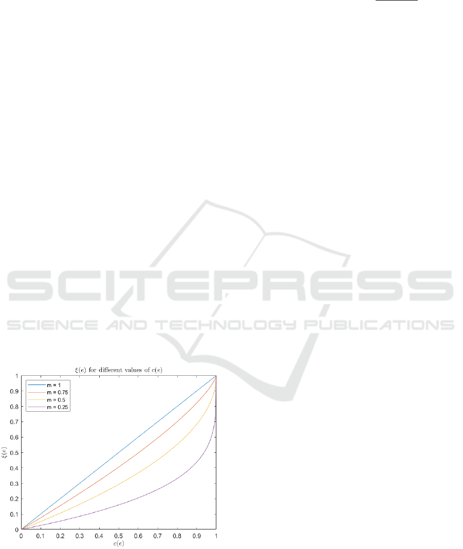
ξ(e) = 1 − exp(m · ln (1 − c(e))) (1)
where c(e) ∈ [0, 1] corresponds to the contrast of an
edge e ∈ E
k
and the multiplier m satisfies m > 0. The
multiplier m controls the skewness of the curve ξ(e)
vs. c(e) as shown in Fig. 2, with different values of
multiplier m. The cost ξ(e) associated with an edge e
is proportional to the contrast c(e). The cost ξ(e) is
bounded between [0, 1] for the different values of c(e)
as follows:
ξ(e) = 0 for c(e) = 0
ξ(e) = 1 for c(e) = 1
ξ(e) ∈ (0, 1) for 0 < c(e) < 1
(2)
The value of the multiplier m adds a non-linear
factor to the cost of the edges. As displayed in Fig.2,
the cost of edges with contrast ranging between (0, 1)
is significantly lower for m = 0.25 as compared to the
cost with multiplier m = 1. The maximum and the
minimum value of the cost ξ(e) remains unaffected
by different values of the multiplier m.
Figure 2: ξ(e) vs. c(e) = [0, 1] for different values of m.
The cost curve β(K ) 7→ R
+
provides the cost as-
sociated with a contraction kernel K = {e
j
∈ E
k
: j ∈
{1, 2, ..., |K |}} for the k
th
level of the graph pyramid
G
k
(E
k
,V
k
):
β(K ) =
|K |
∑
j=1
ξ(e
j
) + λ

|E
k
| − |K |
|E
k
|

(3)
The first term in Equation (3) computes the sum
of the cost associated with all the edges e
j
∈ K . From
Equation (2), the range of the first term
|K |
∑
j=1
ξ(e
j
) is
bounded between [0, |K |]. The second half of the
Equation (3) assists in controlling the kernel size.
Further significance of the second term is made
evident in the explanation of the following objective
function.
Given a set of all the possible contraction kernels S =
{K
1
, K
2
, . . . , K
n
}. The contraction kernel
ˆ
K ∈ S that
helps to select the edges with lower contrast and a
favorable size of contraction kernel is given by:
ˆ
K = arg min
K
i
∈S
β(K
i
) (4)
In Equation (4) we have two parameters: multiplier
m and the Lagrange multiplier λ as shown in Equa-
tions (1,3). From Fig. 2, we can observe that the edges
with a lower contrast have a smaller cost as compared
to the edges with the higher contrast. Hence by mini-
mizing the objective function in Equation (4), we are
giving priority to the edges with the lower contrast,
satisfying the rule mentioned in (Batavia et al., 2020).
The Lagrange multiplier λ penalizes the size of the
contraction kernel. The size of the contraction ker-
nel |K | is directly proportional to λ. Ideally, a larger
contraction kernel is desired as it lowers the height
of the pyramid. In absence of the second term in
Equation (3), the objective function in Equation (4)
might land to a trivial solution with |
ˆ
K | = 1 consist-
ing of a single edge e ∈ E
k
with the lowest contrast. In
the worse case, for a graph G
0
= (V
0
, E
0
) at the base
level, where c(e) = 0 for all edges e ∈ E
0
, this will
result in a pyramid with height |V
0
| and linear com-
plexity for construction of the pyramid (ignoring the
pyramid levels required for the removal of the redun-
dant edges) as in (Cerman et al., 2016). Conversely,
a larger value of λ will result in a larger size of the
contraction kernel, which will eventually reduce the
height of the pyramid (ignoring the pyramid levels re-
quired for the removal of the redundant edges).
Proposition 1. If the edges are selected in the ascend-
ing order of ξ(e), ∀e ∈ E
k
to construct the contraction
kernel K for 0 < |K | ≤ |E
k
|, then the curve |K | vs.
β(K ) will not contain any local maximum.
Proof. The first term
∑
|K |
j=1
ξ(e
j
) of Eq. 3 is a summa-
tion of the edges in ascending order of ξ(e). ξ(e) is
A Step Towards Learning Contraction Kernels for Irregular Image Pyramid
63

bounded between [0, 1] as mentioned in Eq. 2. Hence
the first term of Eq. 3 will result in a convex curve
with no local maximum. The value of the second term
λ

|E
k
|−|K |
|E
k
|

of Eq. 3 is inversely proportional to the
size of the contraction kernel and will result in a linear
curve for 0 < |K | ≤ |E
k
|. The sum of both the terms
will not result in formation of a local maximum. 
As a consequence of Prop. 1, Eq. 4 is eligible for con-
vex optimization.
Algorithm 1 builds an irregular image pyramid
that represents the structure of an image with a graph
of critical vertices on its top level.
Algorithm 1: Objective function based selection of the con-
traction kernel.
1: Input: A 2D image P.
2: Initialize: Generate the 4-connected neighbor-
hood graph G
0
.
3: Insertion of hidden saddle vertices.
4: LBP Categorisation of the vertices into the criti-
cal, non-critical and degenerated vertices.
5: while #(degenerated vertices) >0 do
6: Search for contraction kernel
ˆ
K that optimizes
Equation 4.
7: Set the respective critical vertices as the surviv-
ing vertices and eliminate the edges connecting
two critical vertices from
ˆ
K .
8: Contraction of edges e ∈
ˆ
K .
9: Update the changes in the LBP category of the
degenerated vertices.
10: Simplification of graph by removal of redun-
dant multiple edges.
11: end while
12: while #(non-critical vertices) >0 do
13: Search for contraction kernel
ˆ
K that optimizes
Equation 4.
14: Set the respective critical vertices as the surviv-
ing vertices and eliminate the edges connecting
two critical vertices.
15: Contraction of edges e ∈
ˆ
K .
16: Simplification of graph by removal of redun-
dant multiple edges.
17: end while
18: end
Theorem 2. All the faces at the top level of the pyra-
mid built by Algorithm 1 are slope regions.
Proof. Insertion of the hidden saddles in step 3 of
the Algo. 1 converts all the non-well-composed con-
figurations into well-composed configurations. After
this step, all the faces in the graph are already slope
regions as proven in (Kropatsch et al., 2019)[Proposi-
tion 2]. Now the proof boils down to preserving the
slope regions without changing the connection of the
critical vertices.
For a surface, the topology of its contours changes at
the function value of the critical points. For exam-
ple, the surface contours will collapse to a point at
a non-degenerated extremum and multiple contours
will intersect at a saddle point. In steps 7 and 14
of Algo. 1, we preserve the critical vertices by fix-
ing them as the surviving vertices and preserve the
connection between them by eliminating the edges
connecting two critical vertices. Thus all the edges
selected for contraction belong to a monotonic path
connecting two critical vertices that are not adjacent
to each other. Since the monotonic connections be-
tween the critical vertices are intact, the topology of
the contours will remain the same. Consequently, the
slope regions and the topology of the critical vertices
are preserved. 
4 DICTIONARY FOR THE
CONNECTED COMPONENTS
In this section, we introduce the concept of the dictio-
nary D for the connected components of the contrac-
tion kernel, which comprises sub-graphs conceived as
an element of the contraction kernel. The dictionary is
particularly designed for implementations with com-
binatorial maps as the data structure. The elements
of the dictionary highly depend on the input data, on
the application, and on the the data structure used for
the implementation. Considering Algorithm 1, the
outcome of the algorithm is focused on obtaining the
structure of an image, represented as a graph of criti-
cal vertices. Since the algorithm operates on an irreg-
ular image pyramid, the geometry of the vertices and
edges especially in presence of multiple edges and
self-loops cannot be captured by the adjacency matrix
or adjacency lists. The edge contraction process may
subsequently generate a vertex with a higher degree
and a complex structure bounded by the complexity
of the input data. Therefore, we use combinatorial
maps as the data structure, that implicitly encodes and
characterizes the inclusion relationships.
Combinatorial pyramids (Brun and Kropatsch,
2001) introduced by Brun et. al. is a stack of succes-
sively reduced combinatorial maps. It may be under-
stood as explicit encoding of the edge orientation (ei-
ther in clockwise or anti-clockwise direction) around
the vertex. The combinatorial map M = (D, σ, α) en-
coding consists of three components: (a) a set of darts
D, (b) a permutation σ and (c) an involution α. An
edge e connecting two vertices v, w is composed of
two darts d
1
, d
2
. Darts d
1
and d
2
belonging to the
ICPRAM 2022 - 11th International Conference on Pattern Recognition Applications and Methods
64

same edge e, are related to each other by involution
α such that α(d
1
) = d
2
and α(d
2
) = d
1
. The permuta-
tion σ relates each dart with the following dart around
the same vertex in clockwise or counter-clockwise di-
rection. The direction of encoding is implementation
specific. Fig. 3 displays an example of a simple graph
encoded as a combinatorial map.
Figure 3: An example of a simple graph encoded as a com-
binatorial map.
To maintain generality, the elements of the dictio-
nary are independent of the degree of the vertices and
the geometry of the edges at any level of the pyra-
mid. The elements of the dictionary are differentiated
based on the contraction ratio defined as the reduction
in the number of vertices after contraction of edges in
the connected component C. Table 1 enumerates the
different classes of the connected components C in the
dictionary:
Table 1: Contraction factor for different classes of con-
nected components C in the dictionary D.
|C| contraction factor in |V
k
|
0 1:1
1 2:1
2 3:1
3 4:1
4 5:1
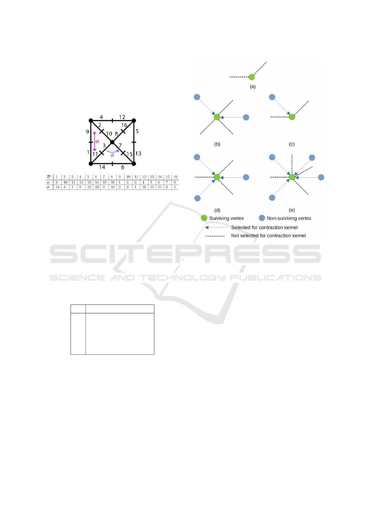
Fig. 4 displays the graphical representation of the
connected components in the dictionary, where the
green vertex represents the surviving vertex and the
blue colored vertex represents the non-surviving ver-
tices. The solid line edges are the edges selected for
the contraction kernel and the dashed lined edges are
excluded from the contraction kernel. The solid line
edges are oriented from the non-surviving vertex to
the surviving vertex, while the dashed line edges are
not oriented. The upper bound on the number of the
dashed line edges is dependent on the complexity of
the data and can be incident to the surviving vertex
Figure 4: Elements of the dictionary D for the connected
component of the contraction kernel.
at various positions apart from the examples shows in
Fig. 4.
Fig.4(a) shows an isolated vertex with respect to
the contraction kernel that does not have any incident
edges selected for contraction operation. A very com-
mon example of an isolated edge is a local extremum
surrounded by other critical vertices. In such configu-
rations, none of the edges are selected for contraction.
Fig.4(b) shows a sub-graph with 1 solid edge se-
lected for the edge contraction and 2 dashed edges
that are not selected for the contraction. After per-
forming the edge contraction on a single edge of
graph G
k
= (V
k
, E
k
), the blue colored vertex will
merge with the green vertex creating a new graph
G
k+1
= (V
k+1
, E
k+1
). The resulting cardinatlity of
edge set and vertex set will be as follows: |E
k+1
| =
E
k
− 1 and |V
k+1
| = V
k
− 1 respectively. The similar
explanation applies for Fig.4(c),(d) and (e).
Following are the remarks and discussion on the
dictionary D:
1. The maximum number of edges selected for the
contraction that is incident on a single vertex is 4.
2. A vertex can either be a surviving vertex or a non-
surviving vertex. The maximum distance between
the surviving vertex of the connected component
and the non-surviving vertices is limited to 1.
A Step Towards Learning Contraction Kernels for Irregular Image Pyramid
65

3. A non-surviving vertex can only have a single
surviving vertex. In other words, a single non-
surviving vertex cannot have multiple surviving
vertices.
The three principal reasons for the above-
mentioned remarks are:
(a) At the base level of the pyramid with graph G
0
, all
the vertices inside the boundary have a degree 4.
(b) Edge contraction operation increases the degree of
the surviving vertex and consequently increases the
complexity for the removal of the redundant edges
(for example: multiple edges and self-loops) for
graph simplification. Therefore, contraction of paths
(as shown in Fig.5) with more than 1 edges are ex-
cluded from the dictionary D. Fig.5(a) shows a sub-
graph with 2 edges e
1
and e
2
selected for the con-
traction. The solid green vertex is the single survivor
of the connected component. We do not consider
bi-colored vertices in our contraction kernels. A bi-
colored vertex is a survivor for edge e
2
and a non-
survivor for edge e
1
. Identifying such paths contain-
ing vertices that act as both survivor and non-survivor
is linear in complexity and requires expensive compu-
tation.
(c) Considering combinatorial maps (Brun and
Kropatsch, 2001) as the data structure for all the el-
ements in the dictionary D, the darts incident on a
single vertex can be easily traversed by computing
the permutations σ starting from a randomly selected
dart incident on the surviving vertex. Conversely, the
process of identifying a path of contraction kernel is
competitively more complicated and time consuming.
Figure 5: Contraction of a path containing more than 1 edge
for contraction, excluded from dictionary D.
5 EXPERIMENTS
This section shows the statistical evidence and ex-
perimental verification of the claims made in Sec-
tion 3. The implementation of the theoretical frame-
work mentioned in this paper can be optimized de-
pending on the application and the data structure in
use. To keep the statistics more general and indepen-
dent of the data-structure, we compared the histogram
of ξ(e) in Equation 1 for different values of multiplier
m for a total of 400 images randomly selected from
the Linnaeus Database (Malmberg et al., 2010). The
size of the images are 32 × 32 (i.e., |E
0
| = 1984) and
the histogram is calculated for ξ(e), ∀e ∈ E
0
of 400
images (1984 ∗ 400 = 793600 edges). For the exper-
iments, the contrast of the edges are normalized with
respect to the maximum contrast of the image, as re-
quired in Eq. 1.
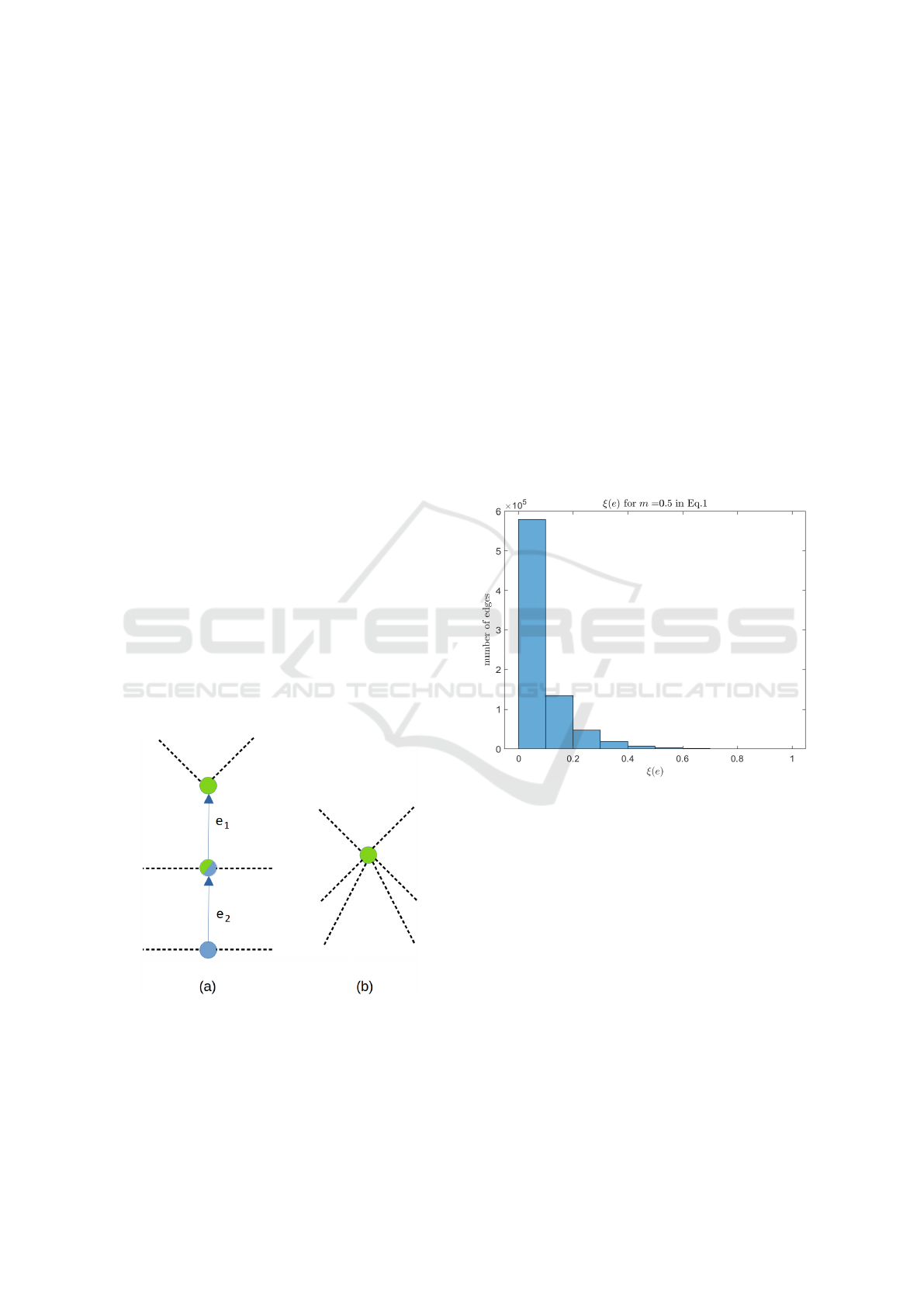
Figure 6: Histogram of ξ(e) for m = 0.5 in Eq.1.
From Fig. 6 we can observe that for m = 0.5, most
of the edges (around 90%) fall in the first two bins
with 0 < ξ(e) < 0.2, while for m = 1 and m = 3 in
Fig. 7,8 there are approximately 75% and 45% of the
edges in the first two bins of ξ(e) histogram respec-
tively. It shows that the multiplier m plays a vital role
in manipulating the contrast of the edges and set the
priority of the edges for the selection process. The
results for m < 0.5 are not displayed due to lack of
visible difference in the histograms. In essence, lower
the value of m, higher number of edges will have low
cost ξ(e) making them eligible for the selection of the
contraction kernel.
Now, let us investigate the cost of the contraction ker-
nel β(K ) as per Eq. 3 for various values of multiplier
m and Lagrange multiplier λ. The graphics displayed
in Fig. 9, 11 were computed for a single gray scale im-
ICPRAM 2022 - 11th International Conference on Pattern Recognition Applications and Methods
66

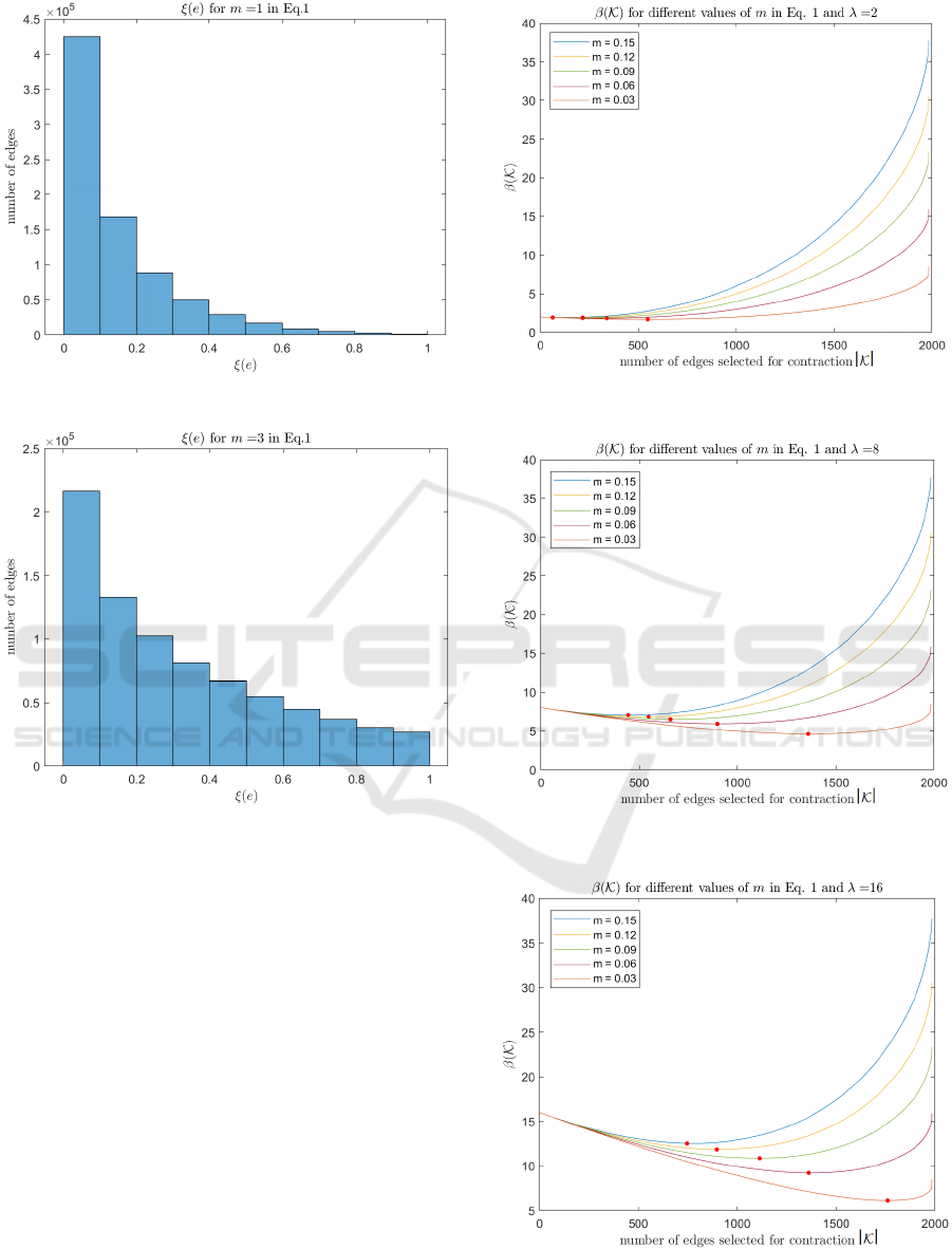
Figure 7: Histogram of ξ(e) for m = 1 in Eq.1.
Figure 8: Histogram of ξ(e) for m = 3 in Eq.1.
age of size 32 × 32 containing 1984 edges in E
0
. The
x-axis represents the size of the contraction kernel |K |
such that the edges are selected in the ascending or-
der of their cost ξ(e) from Eq.1. The red dots mark the
minimum values of the curves.The x-coordinate of the
red dot corresponds to the
ˆ
|K | and the y-coordinate of
the red dot corresponds to the cost of the optimal ker-
nel β(
ˆ
|K |). Each figure contains curves for different
value of m = 0.15,0.12, 0.09, 0.06, 0.03 and a single
value of λ.
On detailed observation of the above graphs and
the corresponding value of ξ(e), ∀e ∈ K , following
were our observations:
1. At the initial stage of the pyramid,
ˆ
K comprises
edges with ξ(e) > 0 i.e. edges that are not a part
of plateau regions and level curves. This is explic-
itly displayed by the orange curve in Fig.11 with
m = 0.03 and λ = 16. The minimum value of the
curve β(K ) is attained at |K | = 1700 edges (ap-
Figure 9: Number of edges selected for the contraction ker-
nel |K | vs. cost of the contraction kernel β(K ) for λ = 2.
Figure 10: Number of edges selected for the contraction
kernel |K | vs. cost of the contraction kernel β(K ) for λ = 8.
Figure 11: Number of edges selected for the contraction
kernel |K | vs. cost of the contraction kernel β(K ) for λ =
16.
A Step Towards Learning Contraction Kernels for Irregular Image Pyramid
67

proximately). As a result there is a higher chance
of the edges with a higher contrast to be selected
for the contraction kernel. This may change the
topology of the image if step 7 and 14 of Algo.1
are not followed. A large size of the contraction
kernel will eventually increase the complexity for
the removal of the edge and graph simplification.
2. For a lower value of λ (typically < 2) and a short
range of 0 < m < 1, the minimum of all the curves
β(K ) for different values of m are very close to
each other and tend to result in the selection of the
same contraction kernel. Fig. 9 is a good example
where only 4 minima are visible because the red
marker for the minimum for curve m = 0.12 and
m = 0.09 coincide each other. Conversely, with a
higher value of λ (typically > 10), we can easily
differentiate between the minimum of the curves
as displayed in Fig. 10,11.
5.1 Estimating the Original Image from
a Blurred Binary Image
In this experiment, we used the proposed method for
estimating the original binary image from its blurred
version utilizing the concept of connected component
labelling (CCL). We assume that the edges present in
the interior of a component will have a lower con-
trast as compared to the edges connecting two distinct
components. By varying the value of the multiplier m
and λ in Eq. 3, we managed to obtain a contraction
kernel containing edges connecting two components
with a small contrast. In Fig. 12, to display an easily
observable and intuitive result, we generated an arti-
ficial image. Fig. 12a shows an image after Gaussian
blur with standard deviation of 0.6 while Fig. 12b dis-
plays CCL with 126 components for m = 0.15 and
λ = 15 and |
ˆ
K | = 76.26% of total edges. By fur-
ther reducing the value of m to 0.05 and increasing
the value of λ to 25, we modify ξ(e) such that higher
number of edges are eligible for the contraction kernel
and |
ˆ
K | = 77.6% of the total edges. As a result the
number of connected components reduce to 66 as dis-
played in Fig. 12c. Repeating the process further, by
lowering m to 0.01 and increasing λ to 45, the number
of edges eligible for contraction raise to |
ˆ
K | = 92.7%,
resulting in 6 connected components corresponding to
the original binary image as shown in Fig. 12d.
The experiments of connected component la-
belling were performed on the YACCLAB database
(Grana et al., 2016). Fig. 13 shows the results
of deblurring MRI binary image from YACCLAB
database. Fig. 13b shows the CCL on the original
image with 1070 connected components. Fig. 13c
and Fig. 13d shows the CCL on the deblurred im-
(a) input image
after Gaussian blur
with std. dev. = 0.6
(b)
#CC = 126 for
m = 0.15 and λ = 15
(c) #CC = 66 for
m = 0.05 and λ = 25
(d) #CC = 6 for
m = 0.01 and λ = 45
Figure 12: Connected component labelling of blurred bi-
nary image with different value of parameter m and λ.
Table 2: Values of parameter m, λ and the resulting number
of connected components for Fig. 12a.
output m λ
number of connected
components (#CC)
Fig. 12b 0.15 15 126
Fig. 12c 0.05 25 66
Fig. 12d 0.01 45 6
ages resulted after tuning the values of m and λ. With
m = 0.01 and λ = 100, we achieved a slight deblur-
ring but the number of connected components were
still high around 12155 as shown in Fig. 13c. With
further fine tuning the values- m = 0.008 and λ = 200,
we achieved a better deblurred image with 2642 num-
ber of connected components (refer Fig. 13d). Table 3
summarizes the results displayed in Fig. 13. From
our observations, the deblurring was not optimal for
higher amount of Gaussian blurring especially when
the small connected components were placed to each
other.
The experiments performed on the YACCLAB
database (Grana et al., 2016) are available: ”click
here” (or visit: https://www.prip.tuwien.ac.at/people/
darshan/more/publications/9 TR.pdf ). The docu-
mented results display both desirable and undesirable
results for connected component labelling and deblur-
ring of binary images.
ICPRAM 2022 - 11th International Conference on Pattern Recognition Applications and Methods
68

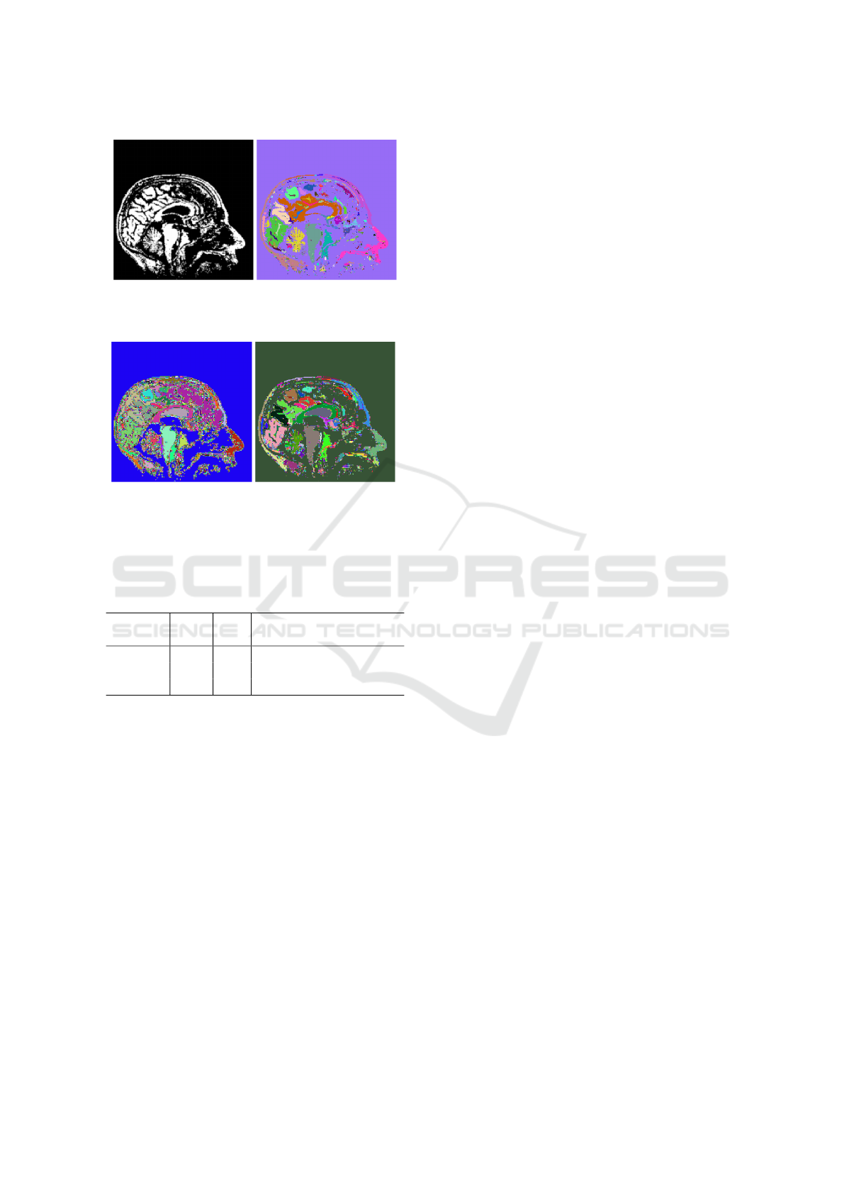
(a) input image
after Gaussian blur
with std. dev. = 0.6
(b) CCL of original image
#CC = 1070 for
m = 0.05 and λ = 90
(c) #CC = 12155 for
m = 0.01 and λ = 100
(d) #CC = 2642 for
m = 0.008 and λ = 200
Figure 13: Connected component labelling of blurred bi-
nary image with different value of parameter m and λ
Table 3: Values of parameter m, λ and the resulting number
of connected components for Fig. 13a.
output m λ
number of connected
components (#CC)
Fig. 13b 0.05 90 1070
Fig. 13c 0.01 100 12155
Fig. 13d 0.008 200 2642
Remarks: We observe that given a dataset of
blurred images, the values of parameter m and λ can
be learned to achieve an optimal deblurring of a test
sample with similar amount of blurring.
As per the TIIP algorithm mentioned (Batavia
et al., 2020), the plateau regions are contracted before
classification of the vertices followed by the contrac-
tion of the edges with c(e) > 0, while preserving the
critical points. Assume we have a 2D image P with R
as the plateau region with the largest diameter d
R
and
C as the gray scale region with the largest diameter d
C
after contraction of R. Then the computational com-
plexity of this algorithm for construction of an irregu-
lar pyramid is O(log(d
R
)+log(d
C
)). With the help of
the objective function we can further reduce the com-
plexity, since we can contract the edges with c(e) > 0
simultaneously with the contraction of the plateau re-
gion. Thus the complexity is reduced to O(log(d
CC
))
where d
CC
corresponds to the diameter of the largest
connected component that may include the gray scale
region C and the plateau region R.
6 CONCLUSIONS
The paper introduces a novel approach for the selec-
tion of the contraction kernel using an objective func-
tion. We proved that the proposed algorithm based
on the objective function navigates the construction
of the irregular pyramid to decompose a 2D image
into monotonically connected image surface regions
(slope regions). The objective function attempts to
replicate the TIIP algorithm mentioned in (Batavia
et al., 2020; Gonzalez-Diaz et al., 2021) and enables
easier modifications for application-oriented results.
It can be envisioned as a step towards learning the
contraction kernel for the construction of an irregu-
lar image pyramid. Later we showed statistical obser-
vations that assist in tuning the parameter values of
the objective function. The experiments were focused
on deblurring of blurred images to recover the origi-
nal binary image and connected component labelling.
Lastly, the paper establishes the concept of the dictio-
nary of the connected components of the contraction
kernel. This dictionary is similar to the dictionary of
the shapes but instead is designed for the graphs es-
pecially considering combinatorial maps as the data
structure. The elements of the dictionary can be used
for the optimization of the objective function and to
realize the solution for the decomposition of an im-
age. We leave the optimization method and the gram-
mar of connected components for future research.
7 FUTURE WORK
The objective function in Equation 4 revolves around
the contrast of an edge. However, it does not help
with the location of the edges in binary images or with
plateau regions, since the contrast of edges belonging
to the same component in a binary image (or plateau
regions) is zero. Edges with same contrast have the
equal priority as per the proposed objective function.
We intend to produce a grammar of the contraction
kernel that repeats its occurrence to deliver an easy
solution. Fig. 14 shows an example of a 9 × 9 grid
like structure of the plateau region such that the solid
and the dashed lines correspond to the edges and the
crossing of the lines correspond to the vertices. All
the edges e have the same contrast c(e) = 0. The set
of the oriented edges form the contraction kernel and
the edges are oriented from the non-surviving vertex
A Step Towards Learning Contraction Kernels for Irregular Image Pyramid
69

to the surviving vertex. The position of the surviving
vertex forms a pattern that corresponds to the knight’s
move in chess. This repetition ensures that the con-
nected components are independent and upon con-
traction, it results in a rotated version of the grid like
structure as shown in Fig.15. The grammar can be
reused on higher levels until the grid structure exists.
Computation of redundant edges, double edges in our
case as shown in Fig.15 can be pre-computed without
an expensive search.
?
?
?
?
?
?
?
?
?
?
?
? ?
?
?
?
?
?
?
?
?
?
?
?
?
? ?
?
?
-
-
-
-
-
-
-
-
-
-
-
-
-
-
-
-
-
-
-
-
-
-
-
-
-
-
-
-
-












 












 

6
6
6
6
6
6
6
6
6
6
6
6
6 6
6
6
6
6
6
6
6
6
6
6
6
6
6 6
6
Figure 14: Knight’s vertex contraction kernel for 9 × 9
plateau region.
Figure 15: After contraction of Knight’s vertex contraction
kernel for 9 × 9 plateau region..
Similar to the graph edit distance, we can com-
pute the pyramid edit distance for an irregular image
pyramid, based on the cost of the contraction kernel
at each level.
REFERENCES
Batavia, D., Gonz
´
alez-D
´
ıaz, R., and Kropatsch, W. G.
(2020). Image = structure + few colors. In Struc-
tural, Syntactic, and Statistical Pattern Recognition
- Joint IAPR Int. Workshops, S+SSPR, LNCS, pages
365–375. Springer.
Batavia, D., Hlad
˚
uvka, J., and Kropatsch, W. G. (2019).
Partitioning 2D Images into Prototypes of Slope Re-
gion. In Int. Conference on Computer Analysis of Im-
ages and Patterns, LNCS, pages 363–374. Springer.
Brun, L. and Kropatsch, W. (2001). Introduction to com-
binatorial pyramids. In Digital and image geometry,
pages 108–128. Springer.
Cerman, M., Janusch, I., Gonzalez-Diaz, R., and Kropatsch,
W. G. (2016). Topology-based image segmentation
using LBP pyramids. Machine Vision and Applica-
tions, 27(8):1161–1174.
Comic, L., De Floriani, L., and Iuricich, F. (2010). Build-
ing Morphological Representations for 2D and 3D
Scalar Fields. In Puppo, E., Brogni, A., and Floriani,
L. D., editors, Eurographics Italian Chapter Confer-
ence 2010, pages 103–110.
Edelsbrunner, H., Harer, J., and Zomorodian, A. (2003). Hi-
erarchical morse-smale complexes for piecewise lin-
ear 2-manifolds. Discrete and computational Geome-
try, 30(1):87–107.
Gonzalez-Diaz, R., Batavia, D., Casablanca, R. M., and
Kropatsch, W. G. (2021). Characterizing slope re-
gions. Journal of Combinatorial Optimization, pages
1–20.
Grana, C., Bolelli, F., Baraldi, L., and Vezzani, R. (2016).
YACCLAB - Yet Another Connected Components La-
beling Benchmark. In 23rd International Conference
on Pattern Recognition. ICPR.
Gyulassy, A., G
¨
unther, D., Levine, J. A., Tierny, J., and
Pascucci, V. (2014). Conforming Morse-Smale Com-
plexes. IEEE Transactions on Visualization and Com-
puter Graphics, 20(12):2595–2603.
Helman, J. L. and Hesselink, L. (1991). Visualizing vector
field topology in fluid flows. IEEE CGA, 11(3):36–46.
Kropatsch, W. G., Casablanca, R. M., Batavia, D., and
Gonzalez-Diaz, R. (2019). On the space between crit-
ical points. In Int. Conference on Discrete Geom-
etry for Computer Imagery, LNCS, pages 115–126.
Springer.
Latecki, L., Eckhardt, U., and Rosenfeld, A. (1995). Well-
composed sets. Comput. Vis. Image Underst., 61:70–
83.
Lee, R. N. (1984). Two-dimensional critical point configu-
ration graphs. IEEE Transactions on Pattern Analysis
and Machine Intelligence, (4):442–450.
Malmberg, G., Nilsson, L.-G., and Weinehall, L. (2010).
Longitudinal data for interdisciplinary ageing re-
search. design of the linnaeus database. Scandinavian
journal of public health, 38(7):761–767.
Morales-Gonz
´
alez, A. and Garc
´
ıa-Reyes, E. B. (2013).
Simple object recognition based on spatial relations
and visual features represented using irregular pyra-
mids. Multimedia tools and applications, 63(3):875–
897.
Shinagawa, Y., Kunii, T., and Kergosien, Y. (1991). Sur-
face coding based on morse theory. IEEE Computer
Graphics and Applications, 11(5):66–78.
Stein, E., Milnor, J. W., Spivak, M., Wells, R., Wells, R.,
and Mather, J. N. (1963). Morse Theory. Princeton
University Press.
ICPRAM 2022 - 11th International Conference on Pattern Recognition Applications and Methods
70