Forecasting Emergency Department Crowding using Data Science

Techniques

Jos

e Manuel Domenech Cabrera

and Javier Lorenzo-Navarro

Insular Maternal-Infant University Hospital Complex of Gran Canaria, Avenida Mar

ıtima del Sur,

s/n., Las Palmas de Gran Canaria, Spain

Inst. of Intelligent Systems and Num. Applic. in Engineering, Univ. of Las Palmas, Las Palmas de Gran Canaria, Spain

Keywords:

Hospital Emergency Department (ED) Predictions, Emergency Department Overcrowding, Time Series

Forecasting, Neural Networks.

Abstract:

The provision of insufﬁcient resources during periods of high demand can lead to overcrowding in emergency

departments. This issue has been extensively addressed through time series forecasting and regression prob-

lems. Despite the fact the increasing number of studies, accurate forecasting of demand remains a challenge.

Thus, the purpose of this study was to develop a tool to predict the future evolution of emergency department

occupancy in order to anticipate overcrowding episodes, avoid their negative effects on health and improve

efﬁciency. This article presents a novel approach under the premise that the ability of the system to drain

patients is the most determining factor in overcrowding episodes as opposed to previous approaches focused

on patient demand. The forecasts model were based on the hourly number of patients occupying the general

Emergency Department of Insular University Hospital of Gran Canaria Island, mainly given data of the ﬂow of

patients through the emergency department as well as performance indicators from other areas of the hospital

extracted from the information system.

1 INTRODUCTION

The application of information technologies in health-

care during the last decade, mainly the implemen-

tation of Electronic Medical Records, has generated

a large volume of health data, making this ﬁeld at-

tractive for scientiﬁc studies as corroborated by the

growth in the number of scientiﬁc publications in re-

cent years (Islam et al., 2018). Data mining is the non-

trivial extraction of implicit, previously unknown in-

formation from the data. Machine learning is a branch

of artiﬁcial intelligence whose goal is to give comput-

ers the ability to learn a task without being explicitly

programmed to perform it. We use the term data sci-

ence to include these techniques and their systematic

application to face some of the current challenges of

healthcare management.

Emergency departments (hereinafter referred to as

ED) are an organization of healthcare professionals

that offers multidisciplinary assistance, located in a

speciﬁc area of the hospital to attend to emergencies

and urgencies. A complete and precise deﬁnition of

acute care can be found in (Hirshon et al., 2013). The

aging of the population (Division, 2019), the chronic-

ity of diseases, together with the sustained increase

over time in the demand for medical care, has aroused

growing concern about the sustainability of the pub-

lic healthcare system (Pammolli et al., 2011). This

situation especially affects emergencies, which is the

fastest growing medical service according to (Min-

istry of Health, 2017), where the provision of insuf-

ﬁcient resources during periods of high demand can

lead to overcrowding. Saturation hinders correct pa-

tient care and causes diagnostic delays, which is re-

lated to an increase in morbidity (Trzeciak and Rivers,

2003), and it also favors human error and increases

mortality (Hoot and Aronsky, 2008). Anticipating

overcrowding would allow us to ensure the quality of

the service, as well as improves efﬁciency, adjusting

resources to the real demand.

This problem can be analyzed from systems the-

ory for a better understanding, trying to model the

different parts of the emergency system and how

changes in some of these parts affect the others. A

conceptual model of (inputs, throughput, output) of

overcrowding is presented in (Asplin et al., 2003) to

understand its causes and develop potential solutions.

The causes of overcrowding in ED have been exten-

504

Domenech Cabrera, J. and Lorenzo-Navarro, J.

Forecasting Emergency Department Crowding using Data Science Techniques.

DOI: 10.5220/0010840700003123

In Proceedings of the 15th International Joint Conference on Biomedical Engineering Systems and Technologies (BIOSTEC 2022) - Volume 5: HEALTHINF, pages 504-513

ISBN: 978-989-758-552-4; ISSN: 2184-4305

 2022 by SCITEPRESS – Science and Technology Publications, Lda. All rights reser ved

sively studied (Derlet and Richards, 2000). Factors

related to saturation can be external or internal to ED.

External pressure is produced by patients visits, this is

stochastic and unplanned, generating a discontinuous

ﬂow determined by multiple factors, such as working

hours, meals, and days of the week. The ﬂow also

varies in holidays, social events, epidemics, climatic

and atmospheric events. Internal causes include in-

sufﬁcient material and human resources or an inad-

equate physical structure. External causes are delay

of radiology and laboratory tests and time required to

ﬁnd a bed for admitted patients (Morley et al., 2018).

An internal pressure is caused by patients who remain

in the department pending complementary tests, ad-

mission and discharge. The availability of beds and

the resolution of complementary tests are at the same

time affected by the demand for the scheduled activ-

ity. When hospital occupancy is high, these demands

compete and the scheduled activity is usually priori-

tized.

Increases in external and internal pressure are the

triggers for overcrowding. Therefore, studying the

historical evolution of these patient ﬂows and their

relationship with previous episodes of overcrowding

can help to predict them. It seems like a suitable

problem for the application of data science techniques

and methods. Measuring the moment in which over-

crowding begins has been object of study, a list of

proposed criteria can be found in (Boyle et al., 2011).

Two of these conditions of overcrowding are the per-

centage of occupancy greater than 100% and the num-

ber of patients waiting for a bed greater than 10%. But

it is not speciﬁed how many of these criteria are suf-

ﬁcient. Furthermore, these criteria should be adapted

to the speciﬁc characteristics of each location. The

number of patient visits or patient arrivals is mostly

used as an indirect indicator of overcrowding because

the service quality is signiﬁcantly related to the pa-

tient demand, but as previously stated, it is only one

of the factors involved. In this research we focus on

the internal performance of the hospital, under the hy-

pothesis that it has a greater impact on the overcrowd-

ing than the patients demand. Thus, we explore some

variables of performance from the ED itself and from

other hospital departments as independent variables

and we use the number of patients occupying the ED

as target variable.

This paper is organized as follows. Section 2 will

review the related works. Section 3 contains the for-

mal description of data, models and experimental set-

tings. Section 4 presents the experimental results, sec-

tion 5 the conclusion.

2 RELATED WORKS

Overcrowding in ED appears to be an universal prob-

lem (Pines et al., 2011) evidenced by the large number

of recent articles that address the problem through a

statistical forecasting approach. An exhaustive review

is presented in (G

ul and Celik, 2018) where the works

are classiﬁed according to the ﬂow of patients (inputs,

throughput, output), the majority of articles focus on

forecasting patient demand, other researchers have

approached this problem by focusing on the charac-

teristics of particular groups of patients, such as in-

ﬂuenza (Araz et al., 2014) and Asthma (Ram et al.,

2015). The frequent throughput objective is the fore-

cast of the length of stays and the forecast of admis-

sions in the case of outputs. Other application themes

includes crowding, utilisation of resources, patient

waiting time, ambulance diversion and inpatient ad-

missions. Our paper does not seem to ﬁt into one of

these three categories since our target variable is re-

lated to all of them, ED occupancy increases with de-

mand raise, in the same way when patient outﬂow and

treatment capabilities decline.

The overcrowding of ED has been extensively ad-

dressed through time series forecasting and regression

problems. Regression is a statistical process to esti-

mate the relationships between a dependent variable

called target and one or more independent continuous

variables, called characteristics. These characteristics

are properties of a phenomenon that is observed, over-

crowding in the problem at hand. When making a

prediction, new characteristic values are provided and

a regression model provides an answer for the target

variable.

Time series is a collection of observations mea-

surements over time and time series forecasting us-

ing mathematical models to forecast the future val-

ues of a series based on previously observed values.

Several techniques have been proposed for time se-

ries forecasting (Hamilton, 1994). These techniques

can be univariate or multivariate, depending on how

many variables are analyzed simultaneously. Accord-

ing to the desired time horizon, it can be short and

long term forecasting. Finally, data can be sampled in

lower or higher frequency. Time series can be decom-

posed into three components. The trend component

is a systematic linear increasing or decreasing of the

series over time. The stationary component are cycles

repeated over time. The noise component are unsys-

tematic ﬂuctuations that cannot be explained by the

model. The linear components of time series is well

explained by classical time series models, unlike non-

linear components. For the latter, modern machine

learning techniques have been proposed.

Forecasting Emergency Department Crowding using Data Science Techniques

505

Most researches uses time series forecasting as

supervised learning, using future time step as la-

bels. Auto-regressive Integrated Moving Average

(ARIMA) (Boyle et al., 2011) models and their vari-

ant SARIMA (Jones et al., 2008) are the most used.

In recent years, the use of modern machine learn-

ing methods such as Artiﬁcial Neural Networks (Gul

and Guneri, 2016), Support Vector Machine (Zlotnik

et al., 2015), Decision Tree (Nas and Koyuncu, 2019),

Random Forest, and Naive Bayes (Hertzum, 2017)

has been incorporated. In recent works, some re-

searchers explore hybrid models, which are the com-

bination of two or more models, expecting to achive

better results comparing with the single model: (Xu

et al., 2016) combines ARIMA and LR in a sequen-

tial manner, because of its ability to capture seasonal

trend and effects of predictors. This model outper-

forms single models in terms of forecasting accuracy.

(Zhang et al., 2019) use a hybrid ARIMA-SVR ap-

proach to forecast daily radiology emergency patient

ﬂow, the hybrid SARIMA-NARNN model to forecast

daily number of admission inpatients is proporsal by

(Zhou et al., 2018). This approach has encouraged us

to explore the use of new hybrid model, our proposal

is to forecast the components separately and assemble

the predictions and compare the results with previous

proposals to evaluate their performance.

The frequency of the data collected and used for

the study most used is daily, followed by monthly

and hourly. Higher frequency time series usually

have more seasonal patterns. Hourly data has daily,

weekly, monthly and annual patterns. Some re-

searchers have shown complications in predicting

hourly patient arrivals (Wargon et al., 2009). More-

over the daily pattern of arrivals is well known and

hourly data show null values. Managers use daily

measurement because overcrowding episodes are not

usually resolved in a few hours. However when use

the census or occupation variable only hourly data has

sense because occupancy can ﬂuctuate during the day.

In addition, we avoid nulls and our forecast can be

more accurate.

The data collection period varied widely, from 1

year to 7 years. In most situations a larger set of

training improves the results of the model. But this is

not always true, it is possible that when adding older

data we will incorporate noise. In some cases, noise

can be easily eliminated, but in other cases there may

be changes in the physical structure of the location

or in the information system that produce trend ﬂuc-

tuations or null values. The forecast horizon ranges

from 1 to 24 hours, from 1 to 30 days and from 1 to

4 months. Most forecast 1 day ahead, which seems

insufﬁcient for resource planning and to avoid over-

crowding episodes. Forecast error generally increase

with the length of the forecast horizon as can be seen

in (Calegari et al., 2016).

We could categorize the variables into the follow-

ing groups: Calendar, Meteorological, Patient and

Miscellaneous. The most used calendar variables are:

weekday, month, holidays and different categories

of holidays. Some works have incorporated meteo-

rological variables such as maximum and minimum

temperature, humidity, wind speed, isolation, rain-

fall, snowfall and pollution. Other data patient used

are gender, triage level, arrival mode, diversion sta-

tus, laboratory orders and radiography orders. Other

miscellaneous variables are google ﬂu trends, ﬂue test

results.

3 MATERIAL AND METHODS

For this work, we have evaluated classic time series

forecasting and machine learning methods, instead of

building a deterministic simulation model of the sys-

tem. We will use the different variables that we can

identify to train a stochastic forecasting model, which

simpliﬁes the construction of the model and we can

discover new relationships and patterns in the data.

As stated before, overcrowding depends on several

variables, so we have faced the problem as multivari-

ate, we have tried different time horizons and sam-

pling frequencies. The general Emergency Depart-

ment of the Insular University Hospital of Gran Ca-

naria Island has been selected for this work. Data of

the ﬂow of patients through the ED as well as perfor-

mance indicators from other areas of the hospital have

been extracted from the information system.

This initial phase focuses on understanding the

project objectives and requirements. The stakeholders

has many competing objectives and constraints that

must be considered. This stage has carried out by lit-

erature review and through interviews with the hospi-

tal managers and domain experts. As a result of these

interviews, a series of improvement objectives were

identiﬁed and a better understanding of the ﬂow of

patients and the care process was obtained, as well as

potential features and data sources were identiﬁed. As

result of the previous literature review, some research

questions were established and an initial assessment

of tools and techniques were performed. The major

research questions we investigate are:

• What insights can be obtained from exploratory

data analysis?

• Can we predict the ED occupation without using

the patient demand?

HEALTHINF 2022 - 15th International Conference on Health Informatics

506

• Can we obtain better results using internal hospi-

tal performance variables?

The major research objectives to achieve are:

• To develop a tool to predict the future evolution of

emergency department occupancy.

• To analyze the correlation of the internal hospital

performance variables with ED overcrowding.

3.1 Data Preparation

The ﬁrst step was to collect the data using Extraction

Transformation and Data Loading (ETL) tools. The

raw data consists of 395.380 rows and 121 columns

that correspond to the patients who have been treated

in the ED from January 1, 2017 to March 1, 2021. As

part of feature engineering process 37 features was

created from raw data grouping by hour and aggre-

gate by the average, resulting 36.933 rows and 38

columns. These features were selected to increase

the predictive power of the learning algorithm, the

full list of features is shown in Table 1. Some of the

attention times have been approximate measured by

taking the time of entry into the information system.

From these features, others are derived by shifting

back rows. This method, called the sliding window, is

used to transform time series into supervised learning

dataset. Count of patients occupying the ED (Census)

is the dependent (target) variable in hourly time se-

ries format. The labels used in the supervised training

were generated by shifting the census series several

hours ahead, the chosen forecast horizon range was

24 to 720 hours. Rows with null values resulting from

shifting were removed and the missing values were

replaced with zeros. other strategies has been tested:

mean, median and k-Nearest Neighbors. Finally, fea-

tures was normalized by scaling each feature between

0 and 1.

Table 1: Features used in the study.

Name Description

time Hourly time stamps.

dayofyear Day of the year from 1 to 365.

dayofweek Day of the year from 1 to 7.

monthofyear Day of the year from 1 to 12.

holiday holiday=1, no holiday=0.

holiday period Laboral=0, christmas=1, sum-

mer=2.

visits Count of arrivals to the ED.

discharge Count of discharges to the ED.

census Count of patients occupying the

ED.

tepcf Minutes elapsed since the patient is

admitted until the ﬁrst medical con-

sultation.

tpu Minutes elapsed since the patient is

admitted until the patient leaves the

ED.

tss Minutes elapsed since the medical

discharge occurs until the patient

leaves the ED.

tssh Minutes elapsed since the medical

discharge occurs until the patient is

admitted to a hospital bed.

tam Minutes elapsed since the start of

the medical consultation until the

medical discharge occurs.

tta Minutes elapsed since the patient

is admitted until the medical dis-

charge occurs.

trc Minutes elapsed since the patient

is admitted until the beginning of

triage.

tc Minutes elapsed since the begin-

ning until the end of the triage.

tpd Minutes elapsed since the patient is

admitted until the ﬁrst diagnosis is

made.

tea Minutes elapsed since the begin-

ning of the triage until the start of

the ﬁrst medical consultation.

tem Minutes elapsed until enter a mod-

ule.

tm Minutes elapsed since the patient

enter a module until the medical

discharge occurs.

tom Minutes elapsed since the patient

enters a module until the patient

leaves the ED.

age Mean age of patients.

level1 level 1 of triage: absolute priority

with immediate attention.

level2 level 2 of triage: very urgent, life-

threatening situations that should

not take more than 10/15 minutes.

level3 level 3 of triage: urgent but clin-

ically stable situation, potentially

life-threatening and with a maxi-

mum delay of 60 minutes.

level4 level 4 of triage: minor urgency

with very low life risk and a max-

imum delay of 120 minutes.

census hosp Count of patients occupying a hos-

pital bed.

sched surg Count of scheduled surgeries.

waiting bed Counting patients waiting for a bed.

traumatology Patient typology.

severe trauma Patient typology.

cardiovascular Patient typology.

gastrointestinal Patient typology.

respiratory Patient typology.

neurologic Patient typology.

codes Patient typology.

psycho social Patient typology.

Forecasting Emergency Department Crowding using Data Science Techniques

507

3.2 Exploratory Data Analysis

Through an exploratory analysis of the data, we can

understand the characteristics of the data which sup-

port the selection of appropriate model. Moreover,

we can also verify our hypothesis about the causes

of overcrowding, concluding if the factors are statis-

tically signiﬁcant. The tool to perform the data anal-

ysis has been Python with libraries pandas, numpy,

matplotlib and seaborn. The hourly census time serie

shown in Fig.1 presents different patterns and high

ﬂuctuations, a signiﬁcant decrease in the census can

be observed during the declaration of the state of

alarm and national lockdown of march 14, 2020 due

to the covid-19 pandemic. Before this moment, a year

stationary pattern can be recognized, for example, the

census decreases in summer and increases in winter.

However, the mean, the standard deviation and the

distribution of values of each year are growing each

year (Table 2). It could indicate that the series was

non-stationary, but this is ruled out by performing the

Augmented Dickey-Fuller unit root test (Dickey and

Fuller, 1979) that can be seen in Table 3. The statis-

tic test value of -13.68 is smaller than the 5% critical

value of -2.86 and p-value is also smaller than signiﬁ-

cant threshold level of 0.05, so we can say the census

time series is stationary and the way it changes re-

mains constant, so it is predictable.

Table 2: Census Statistical Summary.

count mean std min 25% 50% 75% max

Time

2017 8759.0 73.0 26.0 13.0 52.0 69.0 90.0 183.0

2018 8759.0 86.0 27.0 21.0 65.0 83.0 105.0 203.0

2019 8759.0 91.0 32.0 18.0 67.0 89.0 113.0 215.0

2020 8783.0 86.0 37.0 14.0 58.0 82.0 110.0 227.0

2021 1933.0 116.0 34.0 39.0 90.0 112.0 139.0 230.0

Table 3: Results of Dickey-Fuller Test for census serie.

Test Statistic -13.68

p-value 1.37601e-25

Lags Used 24

Number of Observations Used 36968

Critical Value (1%) -3.43

Critical Value (5%) -2.86

Critical Value (10%) -2.57

The histogram of values presented in Fig.2, shows

the bell curve-like shape of the Gaussian distribution

with a longer right tail of outliers. Moreover, the

large difference between 75th percentil and max val-

ues suggests that there are extreme values-outliers in

our data set. Therefore, the data is slightly skewed to

the right, and to eliminate this bias a Box-Cox power

transformation (Box and Cox, 1964) has been applied,

verifying that it slightly improves the results.

A Pearson correlation among features is shown in

Fig.3, Pearson’s coefﬁcient, denoted by the letter r, is

the most commonly reported correlation coefﬁcient.

For non-normal distributions correlation coefﬁcients

should be calculated from the ranks of the data, not

from their actual values. The closer correlation coef-

ﬁcient to 1 indicates a strong and positive correlation

between two features and the correlation closer to 0,

indicate a weak correlation. The closer coefﬁcient to

-1 also implies a strong correlation between the two

series variables but in inverse way. The interpreta-

tion and the name of the correlation strength varies ac-

cording to the authors and the research areas (Akoglu,

2018). We ﬁnd that the correlation rates achieved by

other authors are in ranges similar to ours. The p-

value shows the probability that this strength may oc-

cur by chance, a statistically signiﬁcant heatmap can

be found in Figure 4. Therefore, there are strong cor-

relations with level3, cardiovascular, respiratory and

waiting bed, there are moderate correlations with gas-

trointestinal, level2, neurologic, traumatology, cen-

sus hosp, level4, visits, level1, discharge and psy-

cho social. We notice a moderate inverse correlation

with scheduled surgeries and day number of the week.

Most of these variables have not been used before by

other authors.

The census shifted ahead variables have stronger

correlation with waiting bed than visits, in addition

census hosp and visits have the same strength. This

fact veriﬁes our hypothesis about the higher inﬂuence

of the hospital performance compared to external de-

mand. Other performance variables are strongly cor-

related, especially patient typologies and emergency

levels, we notice that cardiovascular and respiratory

variables are stronger correlated than other categories,

we also notice that level3 is more correlated than other

more critical levels.

Time series can be be analyzed through the de-

composition of its time series components, hourly

census decomposed by the additive model is shown

in Figure 5. The Trend does not show long term pos-

itive or negative tendency in hourly frequency, how-

ever there is an annual growing trend. The Seasonal

indicates a strong hourly pattern that also occurs daily,

weekly and annually. Therefore, we expect that mod-

els suitable for multivariate time series with trend and

multiple seasonal components will reach better re-

sults.

The ACF (Auto-Correlation Function) gives us

auto-correlation measures of the series with its lagged

values and PACF (Partial Auto-Correlation Function)

give us auto-correlation measures of the residuals,

HEALTHINF 2022 - 15th International Conference on Health Informatics

508

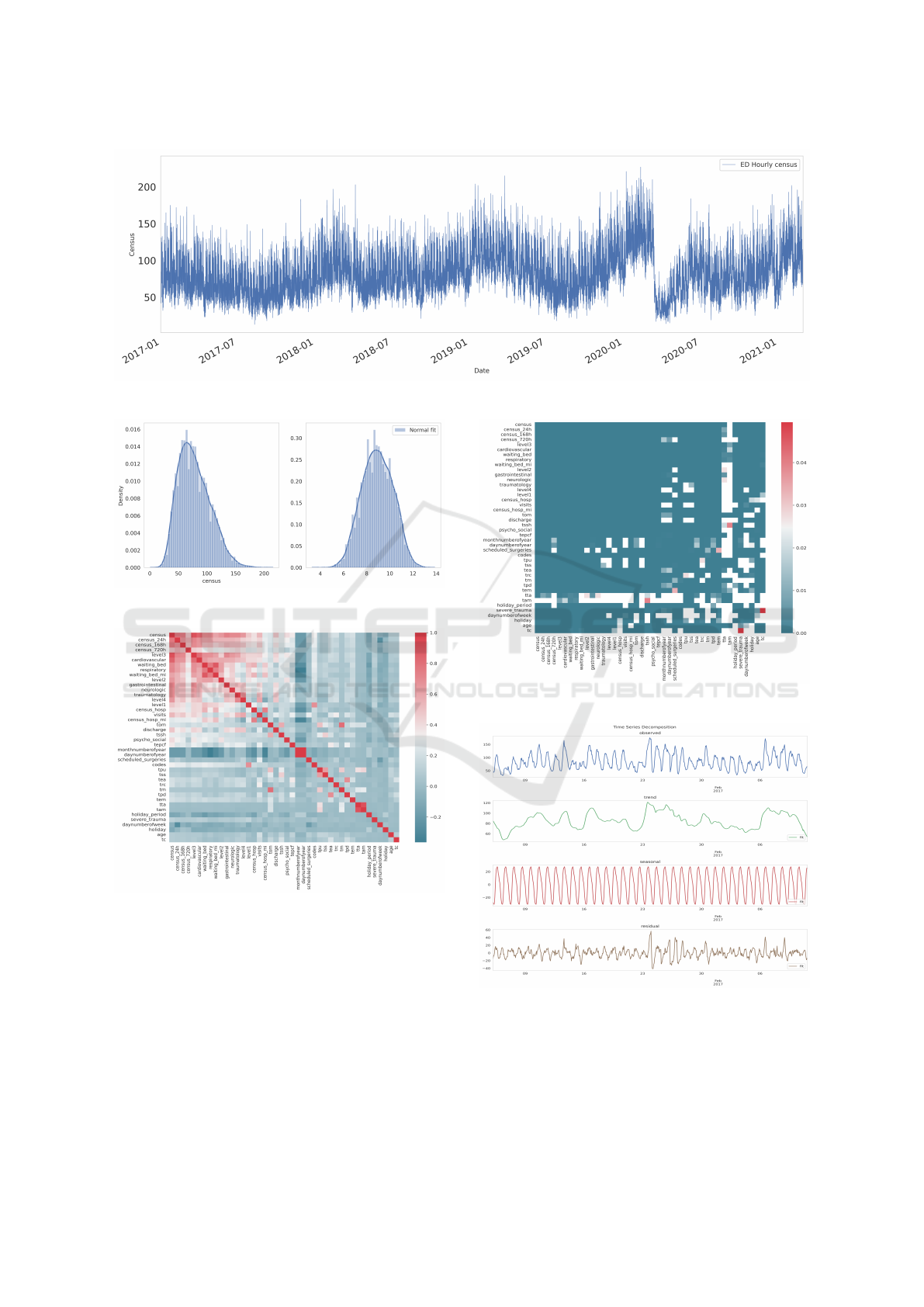
Figure 1: ED hourly census time serie.

Figure 2: ED hourly census and normal ﬁt census.

Figure 3: Correlation heatmap.

which remains after removing the seasonally and

trend effects. ACF and PACF in Figure 6 show peaks

that coincide with the seasonality daily period.

3.3 Experimental Design and

Implementation

Several models have been selected from the litera-

ture review. The selection includes the models fre-

quently applied in this problem, and others that have

Figure 4: Statistically signiﬁcant correlation.

Figure 5: ED hourly census decompose.

exhibited good results applied to other forecasting and

regression problems with time series. Different lin-

ear regression models have been compared to analyze

the correlation of the internal hospital performance

variables with ED overcrowding. Those linear meth-

Forecasting Emergency Department Crowding using Data Science Techniques

509

Figure 6: Auto-Correlation function.

ods are: standard linear regression (Standard), Ridge

regression that includes the L2 regularization of the

weights, Lasso optimization that includes the L1 reg-

ularization of the weights increasing the number of

non-zero coefﬁcients, and a combination of Ridge and

Lasso named Elastic-Net that includes L1 and L2 reg-

ularization.

Before the dataset was split into training dataset

(80%) and testing dataset (20%) a process of fea-

ture selection was tested to reduce the number of fea-

tures by selecting the most signiﬁcant. Feature se-

lection reduces training time and can improve accu-

racy (Piramuthu, 2004). We have implemented fea-

ture selection through SelectFromModel method from

sklearn library, a meta-transformer for selecting fea-

tures based on importance weights. The selection

has been made on the set of variables shown in Ta-

ble1. The inclusion in the set of the variables derived

from these by the sliding window method also has

been tested. All the tests we have performed of au-

tomatic feature selection have generated models with

larger error scores than the exhaustive manual selec-

tion method. This means that the selection method is

leaving out important variables. The set of features

selected by exhaustive process is shown in Table 4.

Different linear time window sizes have been tested

obtaining optimal performance with 168 lags. The

deﬁnitive set contains 3024 features derived from pre-

vious inputs of each of these 18 features by the sliding

window method.

4 RESULTS AND DISCUSSION

To assess the performance of the methods, the follow-

ing measures are the most widely used: Mean Abso-

Table 4: Features selected.

Name Description

dayofyear Day of the year from 1 to 365.

dayofweek Day of the year from 1 to 7.

holiday holiday=1, no holiday=0.

holiday period Laboral=0, christmas=1, sum-

mer=2.

discharge Count of discharges to the ED.

visits Count of arrivals to the ED.

census Count of patients occupying the

ED.

tepcf Minutes elapsed since the patient is

admitted until the ﬁrst medical con-

sultation.

tssh Minutes elapsed since the medical

discharge occurs until the patient is

admitted to a hospital bed.

trc Minutes elapsed since the patient

is admitted until the beginning of

triage.

level1 level 1 of triage: absolute priority

with immediate attention.

level2 level 2 of triage: very urgent, life-

threatening situations that should

not take more than 10/15 minutes.

level3 level 3 of triage: urgent but clin-

ically stable situation, potentially

life-threatening and with a maxi-

mum delay of 60 minutes.

level4 level 4 of triage: minor urgency

with very low life risk and a max-

imum delay of 120 minutes.

census hosp Count of patients occupying a hos-

pital bed.

waiting bed Counting patients waiting for a bed.

cardiovascular Patient typology.

respiratory Patient typology.

neurologic Patient typology.

lute Percentage Error (MAPE), Root Mean Square Er-

ror (RMSE), Mean Absolute Error (MAE), and coef-

ﬁcient of determination (R-squared). Good accuracy

is reached when the differences between the observa-

tions and the predicted values are small and unbiased.

MAPE is the mean of the difference between the ob-

servations and the predicted, expressed as a percent-

age of the observations. Lower values indicate better

model performance. It is used frequently for its easy

interpretation. However, MAPE divides each error by

the demand, so high errors during low-demand peri-

ods have a great impact. It is not a good measure to

optimize a model because it will undershoot the de-

mand. RMSE is the root squared mean of the squared

differences between predicted and actual values. It

gives more importance to the most signiﬁcant errors,

its version without square root MSE has been selected

as regression loss function. MAE has easy interpre-

tation and is less sensitive to outliers. R-squared is

HEALTHINF 2022 - 15th International Conference on Health Informatics

510

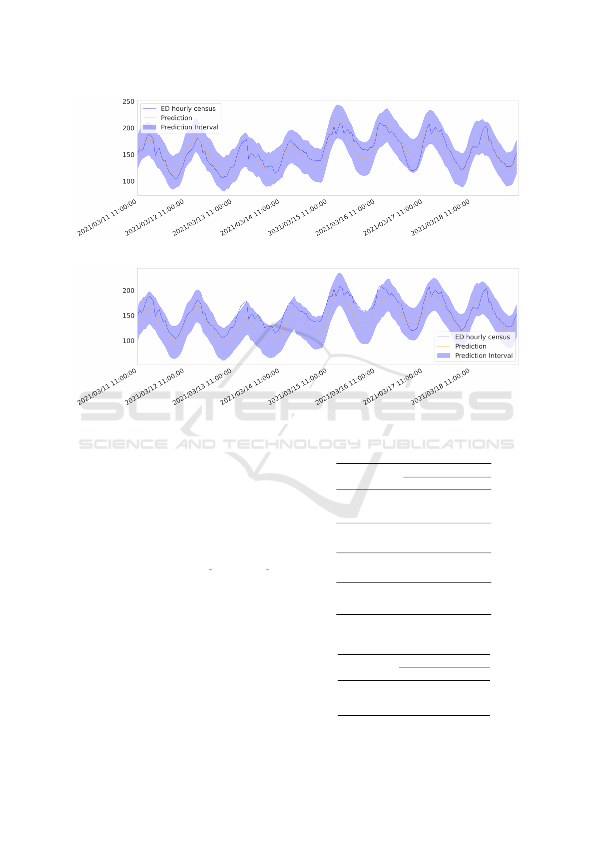
Figure 7: ED hourly census prediction 24 hours ahead with performance variables.

Figure 8: ED hourly census prediction 24 hours ahead without performance variables.

the percentage of explained variability by the model.

Unlike the previous ones, it is unscaled and a higher

R-squared value means a better model accuracy.

Table 5 shows the results obtained with the com-

pared regression methods and it can be observed that

all of them perform similarly. As expected, the fore-

cast accuracy decreases as the time horizon go ahead.

Figure 7 shows the predicted census 24 hours ahead

by standard Linear Regression method and prediction

interval with 95% of conﬁdence.

To assess the signiﬁcance of the internal hospi-

tal performance variables: census

hosp, waiting bed,

tepcf, tssh, and trc; an ablation study was carried out

removing those variables from the model. Table 6

shows the results and it can be noted a decrease in the

performance in all conﬁgurations, except for MAPE

and 1-day ahead horizon, this can be seen in Figure 8,

it can be observed that this model is a worse ﬁt for the

real census.

Table 5: Occupancy forecast using linear models and

performance variables.

Method Horizon Test error

MAERMSE MAPE R

Standard 1 day 12.64 15.89 12.70%0.81

1 week 17.42 22.48 17.10%0.62

1 month20.86 26.72 19.52%0.46

Lasso 1 day 12.73 16.03 12.80%0.81

1 week 17.45 22.48 17.13%0.62

1 month20.88 26.74 19.50%0.46

Ridge 1 day 12.64 15.89 12.70%0.81

1 week 17.42 22.48 17.10%0.62

1 month20.86 26.72 19.52%0.46

ElasticNet1 day 12.72 16.03 12.80%0.81

1 week 17.45 22.49 17.13%0.62

1 month20.88 26.74 19.50%0.46

Table 6: Occupancy forecast using linear regression

without performance variables.

Method Horizon Test error

MAERMSE MAPE R

Standard1 day 13.45 17.34 12.38% 0.77

1 week 23.90 31.04 20.88% 0.27

1 month29.72 39.60 24.97%-0.18

Forecasting Emergency Department Crowding using Data Science Techniques

511

5 CONCLUSIONS

We can now answer the research questions raised in

section3.

• What insights can be obtained from exploratory

data analysis?: The exploratory analysis of the

data shows us a higher predictive value of the in-

ternal performance variables. The dependent vari-

able has a stronger correlation with waiting bed

than visits, and census hosp and visits have the

same strength. This fact veriﬁes our hypothesis

about the higher inﬂuence of the hospital perfor-

mance compared to external demand. Other vari-

ables are stronger correlated, especially patient ty-

pologies and critical levels. We notice that car-

diovascular and respiratory variables are stronger

correlated than other categories, we also notice

that level3 is more correlated than other more crit-

ical levels.

• Can we predict the ED occupation without us-

ing the patient demand? Although the inﬂuence

of hospital performance is very important, we

achieved better results by characterizing all fac-

tors related to overcrowding, both external and in-

ternal.

• Can we obtain better results using internal hos-

pital performance variables? Deﬁnitely, incorpo-

rating the proposed variables improves the results

of the ED overcrowding forecasting models.This

has been conﬁrmed with the ablation study where

these variables were eliminated and the perfor-

mance of the estimation decreased.

All the research objectives have been reached, the

results show that ED occupation can be predicted

from internal performance variables, even excluding

external demand. A better understanding of the corre-

lation of internal hospital performance variables with

overcrowding in emergency departments has been

reached.

The linear regression models used in the experi-

ments are powerful enough to yield good performance

but not so much complex to mask the inﬂuence of the

variables in the results. Thus, they allow us to estab-

lish a baseline for future works to explore the use of

different machine learning models like artiﬁcial neu-

ral networks and decisions trees. Another possible fu-

ture work is to explore the use of exogenous variables.

REFERENCES

Akoglu, H. (2018). User’s guide to correlation coefﬁcients.

Turkish Journal of Emergency Medicine, 18(3):91–93.

Araz, O., Bentley, D., and Muelleman, R. (2014). Us-

ing google ﬂu trends data in forecasting inﬂuenza-

like–illness related emergency department visits in

omaha, nebraska. The American Journal of Emer-

gency Medicine, 32.

Asplin, B. R., Magid, D. J., Rhodes, K. V., Solberg, L. I.,

Lurie, N., and Camargo, C. A. (2003). A conceptual

model of emergency department crowding. Annals of

Emergency Medicine, 42(2):173–180.

Box, G. E. P. and Cox, D. R. (1964). An analysis of trans-

formations. Journal of the Royal Statistical Society.

Series B (Methodological), 26:211–252.

Boyle, J., Jessup, M., Crilly, J., Green, D., Lind, J., Wal-

lis, M., Miller, P., and Fitzgerald, G. (2011). Predict-

ing emergency department admissions. Emergency

medicine journal : EMJ, 29:358–65.

Calegari, R., Fogliatto, F., Lucini, F., Neyeloff, J., Kuchen-

becker, R., and Schaan, B. (2016). Forecasting daily

volume and acuity of patients in the emergency de-

partment. Computational and Mathematical Methods

in Medicine, 2016:1–8.

Derlet, R. W. and Richards, J. R. (2000). Overcrowd-

ing in the nation’s emergency departments: Complex

causes and disturbing effects. Annals of Emergency

Medicine, 35:63–68.

Dickey, D. and Fuller, W. (1979). Distribution of the esti-

mators for autoregressive time series with a unit root.

JASA. Journal of the American Statistical Association,

74.

Division, P. (2019). World population ageing: highlights.

New York : UN, 2019, page 37.

ul, M. and Celik, E. (2018). An exhaustive review and

analysis on applications of statistical forecasting in

hospital emergency departments. Health System.

Gul, M. and Guneri, A. (2016). Planning the future of emer-

gency departments: Forecasting ed patient arrivals by

using regression and neural network models. Inter-

national Journal of Industrial Engineering: Theory,

Applications and Practice, 23:137–154.

Hamilton, J. (1994). Time series analysis. Princeton Univ.

Press, Princeton, NJ.

Hertzum, M. (2017). Forecasting hourly patient visits in the

emergency department to counteract crowding. The

Ergonomics Open Journal.

Hirshon, J., Risko, N., Calvello, E., Ramirez, S., Narayan,

M., Theodosis, C., and O’Neill, J. (2013). Health sys-

tems and services: The role of acute care. Bulletin of

the World Health Organization, 91:386–388.

Hoot, N. and Aronsky, D. (2008). Systematic review of

emergency department crowding: Causes, effects, and

solutions. Annals of emergency medicine, 52:126–36.

Islam, M. S., Hasan, M. M., Wang, X., Noor-E-Alam, M.,

and Germack, H. (2018). A systematic review on

healthcare analytics: Application and theoretical per-

spective of data mining. Healthcare, 6.

Jones, S., Thomas, A., Evans, R. S., Welch, S., Haug, P.,

and Snow, G. (2008). Forecasting daily patient vol-

umes in the emergency department. Academic emer-

gency medicine : ofﬁcial journal of the Society for

Academic Emergency Medicine, 15:159–70.

HEALTHINF 2022 - 15th International Conference on Health Informatics

512

Ministry of Health, S. (2017). Siae emergency activity. Sta-

tistical Portal of the National Health System.

Morley, C., Unwin, M., Peterson, G., Stankovich, J., and

Kinsman, L. (2018). Emergency department crowd-

ing: A systematic review of causes, consequences and

solutions. PLOS ONE, 13.

Nas, S. and Koyuncu, M. (2019). Emergency department

capacity planning: A recurrent neural network and

simulation approach. Computational and Mathemati-

cal Methods in Medicine, 2019:1–13.

Pammolli, F., Riccaboni, M., and Magazzini, L. (2011). The

sustainability of european health care systems: Be-

yond income and aging. The European journal of

health economics : HEPAC : health economics in pre-

vention and care, 13:623–34.

Pines, J., Hilton, J., Weber, E., Alkemade, A., Shabanah,

H., Anderson, P., Bernhard, M., Bertini, A., Gries, A.,

Ferrandiz, S., Kumar, V., Harjola, V.-P., Hogan, B.,

Madsen, B., Mason, S., Ohl

en, G., Rainer, T., Rath-

lev, N., Revue, E., and Schull, M. (2011). Interna-

tional perspectives on emergency department crowd-

ing. Academic emergency medicine : ofﬁcial jour-

nal of the Society for Academic Emergency Medicine,

18:1358–70.

Piramuthu, S. (2004). Evaluating feature selection methods

for learning in data mining applications. European

Journal of Operational Research, 156:483–494.

Ram, S., Zhang, W., Williams, M., and Pengetnze, Y.

(2015). Predicting asthma-related emergency depart-

ment visits using big data. IEEE journal of biomedical

and health informatics, 19.

Trzeciak, S. and Rivers, E. (2003). Emergency depart-

ment overcrowding in the united states: An emerging

threat to patient safety and public health. Emergency

medicine journal : EMJ, 20:402–5.

Wargon, M., Guidet, B., Hoang, T., and Hejblum, G.

(2009). A systematic review of models for forecasting

the number of emergency department visits. Emer-

gency medicine journal : EMJ, 26:395–9.

Xu, Q., Tsui, K.-L., Jiang, W., and Guo, H. (2016). A hybrid

approach for forecasting patient visits in emergency

department: Forecasting patient visits. Quality and

Reliability Engineering International, 32:2751–2759.

Zhang, Y., Luo, L., Yang, J., Liu, D., Kong, R., and Feng, Y.

(2019). A hybrid arima-svr approach for forecasting

emergency patient ﬂow. Journal of Ambient Intelli-

gence and Humanized Computing, 10:3315–3323.

Zhou, L., Zhao, P., Wu, D., Cheng, C., and Huang, H.

(2018). Time series model for forecasting the number

of new admission inpatients. BMC Medical Informat-

ics and Decision Making.

Zlotnik, A., Gallardo-Antol

ın, A., Cuchi, M., P

erez, M.,

and Montero, J. (2015). Emergency department visit

forecasting and dynamic nursing staff allocation us-

ing machine learning techniques with readily available

open-source software. Computers, informatics, nurs-

ing : CIN, 33.

Forecasting Emergency Department Crowding using Data Science Techniques

513

REFERENCES

Akoglu, H. (2018). User’s guide to correlation coefficients.