
Image Coding by Samples of Counts as an Imitation of the Light
Detection by the Retina
V. A. Kershner and V. E. Antsiperov
a
Kotelnikov Institute of Radioengineering and Electronics of RAS, Mokhovaya 11-7, Moscow, Russian Federation
Keywords: Image Representation, Photon-Counting Sensor, Ideal Imaging Device, Ideal Image Concept, Counting
Statistics.
Abstract: The results of the study of a new method of image coding based on samples of counts are presented. The
method is based on the concept of an ideal image, motivated by the mechanisms of light perception by the
retina. In this regard, the article discusses general statistical issues of the interaction of radiation with matter
and based on a semiclassical approach, formalizes the concepts of an ideal imaging device and an ideal image
as a point Poisson 2D-process. At the centre of the discussion is the problem of reducing the dimension of an
ideal image to a fixed (controlled) size representation by a sample of counts. The results of illustrative
computational experiments on counting representation/coding of digital raster images are also presented.
1 INTRODUCTION
In the human visual system, the radiation (light)
coming from the outside World is registered by the
special cells called photoreceptors. These cells are the
main components of the outer layer of the retina, see
Figure 1, and are divided into rods, cylindrical cells,
and cones having a conical shape. It is these two types
of photoreceptors that allow the visual system to
receive primary information in the form of light
radiation from the outside. The usefulness of such
data is due to most objects around us, even though
they themselves are not sources of light radiation,
reflect light from other sources quite well, depending
on their characteristics, such as surface structure,
shape, luminosity and others.
Figure 1: Scheme of the human eye with retina, based on
which the data about objects of the external World are
transformed into internal Visual system representations.
a
https://orcid.org/0000-0002-6770-1317
The methods of registration and primary
processing of optical radiation in the visual system
began to be actively used already since the XVIII
century, after the discovery of photochemical
reactions by Wilhelm Homberg in 1694. However,
the first cameras appeared much earlier, it is known
that back in the V century BC, the ancient Chinese
philosopher Mo-Tzu described the action of a pinhole
camera, the simplest device that allows you to obtain
an optical image of objects. To date, image
registration and transformation systems have been
improved, and with them, the number of borrowed
mechanisms of the visual system has grown. It is
worth noting several common borrowings, such as the
use of an optical focusing system presented in the
visual system in the form of a lens, a diaphragm
(pupil), as well as a variety of sensitive elements
(photoreceptors) registering radiation, ranging from
the simplest transparent and translucent films and
plates with a photosensitive mixture applied to the
surface, and ending with high-tech CCD/CMOS
photodiodes. Some features of the eye, such as the
presence of a vitreous body between the lens and
photoreceptors, the shape of the retina (the
photosensitive surface of the eye) in the form of a
hollow ball, not a plane, etc. are not essential in this
context.
Kershner, V. and Antsiperov, V.
Image Coding by Samples of Counts as an Imitation of the Light Detection by the Retina.
DOI: 10.5220/0010836800003122
In Proceedings of the 11th International Conference on Pattern Recognition Applications and Methods (ICPRAM 2022), pages 41-50
ISBN: 978-989-758-549-4; ISSN: 2184-4313
Copyright
c
2022 by SCITEPRESS – Science and Technology Publications, Lda. All rights reserved
41
The use of visual perception mechanisms in
artificial systems was best manifested in the
registration of light radiation. It is worth
remembering such discoveries as daguerreotype, a
technology for the manifestation of a weak latent
image using mercury vapor, developed by Daguerre
in 1837, and his developments - silver-coated plates,
which by the 20th century had been improved to
celluloid photographic films with gelatin-silver
emulsion, which was the beginning of analog
photography. And by the beginning of the XXI
century, with the development of technologies, the
registration of light radiation moved to a new level,
digital photography appeared, which was based on
photodiode arrays registering radiation. To a large
extent, these successes were provided by the
invention of a charge-coupled device (CCD) in 1969
by Willard Boyle and George Smith and the further
invention of photosensitive matrices on
complementary metal-oxide-conductor (CMOS)
structures. In 1993 the team of Eric Fossum
developed the first CMOS sensor of active pixels. The
transition from analog photography to digital one has
made it possible to improve several parameters of
photo and video cameras, of particular importance
among which is an increase in spatial resolution,
which resulted from a reduction in the size of
photodetectors down to several microns. It is also
worth mentioning other achievements related to the
development of digital technologies, such as reducing
power consumption, increasing frame rate, etc.
Let us note, that the technological achivements
listed above are essentially related to the scientific
developments of the XX century, in particular, such
branches of science as quantum electrodynamics (the
interaction of radiation with matter) (Fox, 2006) and
solid-state theory (the development of semiconductor
structures) (Holst, 2011).
Modern ideas indicate that along with the
progressive decrease in the size of photodetectors of
digital matrices, the nature of radiation registration
also changes, acquiring a pronounced quantum
character, allowing the sensors to work in the so-
called mode of counting single photoelectrons. To
date, the registration of individual photons has
already been achieved by several modern
technologies, such as photon-counting Image Sensors
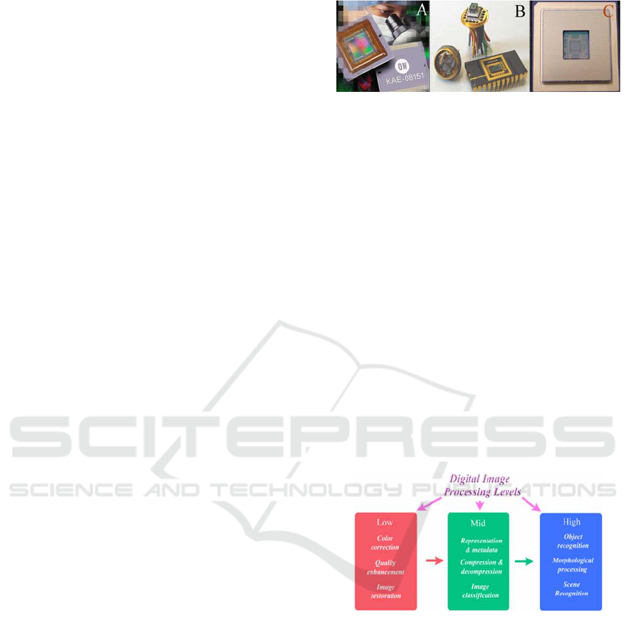
(Fossum, 2017). It is also worth mentioning the
variety of such sensors represented by electron-
multiplying matrices with charge capacity (EMCCD)
(Robbins, 2011), single-photon avalanche diodes
(SPAD) (Dutton, 2016), avalanche photodiodes in
Geiger counter mode (GMAPD) (Aull, 2015), see
Figure 2.
Figure 2: Modern photon-counting sensor technologies
based on A) EMCCD, B) SPAD, C) GMAPD.
Since photons are transformed into the electric
current from the digital video-matrix of photodiodes,
the last can be easily included in various electronic
circuits, which, in turn, may contain microprocessors
necessary for digital signal processing (DSP).
Taking into account the high efficiency of modern
microprocessors, it becomes possible to solve not
only a standard set of video signal preprocessing tasks
related to glare compensation, dark current, white
balance, but also to perform significantly complex
operations comparable to those that occur in the
human brain - pattern recognition, event analysis,
classification of images by features, etc. Such a
possibility opens up new opportunities in the
formation, processing, and analysis of images based
on digital image signal processing (DISP) methods.
In turn, the modern DISP theory (Gonzalez, 2007)
provides digital video data recording devices with a
number of tools and methods for processing visual
information, see Figure 3.
Figure 3: A rough diagram of modern digital image signal
processing (DISP).
Conventionally, all methods aimed at processing
digital images can be divided into three main types –
computerized processes of the low, medium, and high
level (Figure 3). The first level of processes usually
includes operations related to the preprocessing of
input data. These include noise reduction, quality
correction, contrast improvement, etc. The second
level consists of procedures for segmentation,
classification of images by common features,
recognition of individual elements, and bringing them
into a form convenient for possible further computer
processing. And finally, the third level of processing
covers tasks such as semantic analysis of recognized
ICPRAM 2022 - 11th International Conference on Pattern Recognition Applications and Methods
42

objects and scenes. In other words, high-level
processing implies some "comprehension" of what
was recorded in the image, which can be associated
with human vision.
It should be noted that some mechanisms of the
human visual system are also actively used at all
levels of the DISP (Gabriel, 2015). At the same time,
each of the three levels can be correlated with the
corresponding elements of the visual system. The
methods of the first level are characterized by the
mechanisms of preprocessing registered data in the
retina. The third level contains the methods that
simulate some brain processing of input data
mechanisms. The last are associated with serious
work in the cerebral cortex (Rodieck, 1998), in this
connection, it is worth highlighting machine learning
methods (Barber, 2012), such as object and scene
recognition, morphological analysis, etc. As for the
methods of the second group, they occupy a median
value between the first and third levels and are
probably implemented by the visual system also in
the area between the retina and the cerebral cortex
itself.
It should be noted that, despite the current level of
technological achievements, the use of visual
perception mechanisms in artificial imaging systems
is implemented within the DISP with a certain degree
of approximation. Already at the level of
representation of registered data, approximate
modeling is used, since most traditional DISP
methods are focused on raster (bitmap) images
representing discrete pixels – the digitized result of
the accumulated energy of the radiation recorded by
the detectors during the exposure time. In other
words, the pixel values are proportional to the total
number of photons registered by the sensitive areas of
the corresponding matrix detectors. In the case of the
retina, photoreceptors react rather to individual
photons of radiation, transmitting a count signal to the
ganglion cells of the inner layer instantly, without the
accumulation (Rodieck, 1998). This difference in the
representation of input data in natural and artificial
video systems is a consequence of the fact that until
recently, the technological capabilities for
implementing image registration methods similar to
those occurring in the visual system were simply
absent. Fortunately, significant progress has been
made in recent decades in the development of
photodiode matrices operating in the mode of
counting single photons (see also (Morimoto, 2020)).
It opens new opportunities for the DISP methods,
modeling the processes of registering visual data in
the retina. One of the possible approaches to
developing this problem is presented below as a new
method of encoding (representing) images with
samples of counts simulating the mechanism of
registering radiation in the human visual system.
2 IMAGE CODING BY SAMPLES
OF COUNTS
To substantiate the method of coding (representation)
of visual data (images), first of all, it is worth
considering the processes of light radiation
registration by photosensitive elements of the human
visual system. The following discussion is justified
by widely known biophysical facts about the
interaction of radiation with photoreceptor cells of the
retina (Rodieck, 1998) and are also motivated by the
provisions of quantum electrodynamics (Fox, 2006)
at least in its semi-classical approximation (Goodman,
2015). All results will be further formalized in the
form of a general model of an ideal image (Pal, 1991),
which is recorded by an ideal imaging device,
containing a huge array of point photodetectors
(Antsiperov, 2021).
As mentioned above, the primary device in the
human imaging pipeline is the retina. To substantiate
the adequacy of retina model used below, it is worth
mentioning several key facts concerning it. It is well
known that the retina of the human eye includes about
100 million rods and 10 million cones capable of
registering individual photons of the visible spectrum
of light radiation. The density of these photoreceptors
varies from 100 to 160 thousand receptors per mm
2
(in some living creatures, this parameter may be
significantly higher, for example, in birds of prey,
there are about a million photoreceptors per square
millimetre of the retina). At the same time, it is worth
noting that the signals coming to the cerebral cortex
via the optic nerve are (see Figure 1) not the same data
that were received by photoreceptors. These signals
are formed from receptors by the upper layer of cells
of the retina of the eye, undergoing processing in a
complex system of cells of the middle and inner
layers. At the final stage, visual information entering
the cerebral cortex is transmitted along the optic
nerve –axons of ganglion cells. Their number is about
a million, which is about two orders of magnitude less
than the number of photoreceptors.
The prototype of the imaging device for forming
an ideal image, which can also be perceived as a
technical implementation of the latter, can be selected
in the form of a matrix of single-photon avalanche
diodes (SPAD) (Morimoto, 2020), or any of its
analogues (Fossum, 2017). The production of such
Image Coding by Samples of Counts as an Imitation of the Light Detection by the Retina
43

matrices currently allows to get amazing results –
about a million micro-detectors of light radiation are
placed on a surface of 120 mm
2
in pitch of 9.4
microns. Each detector has a dynamic binary memory
for storing registered data and has a memory refresh
rate of 24 thousand frames per second (Morimoto,
2020). From where the flow of information from the
SPAD matrix of photodiodes is easily estimated. If
the information flow in the human visual system is
approximately 50 Mbit/sec, then the information flow
of the matrix of single-photon avalanche diodes
reaches 25 Gbit/sec (Koch, 2006).
Despite the difference between artificial and
natural mechanisms of forming an image, they all
have common features. Both have a finite 2D-
dimensional photosensitive region containing a huge
number of receptors / photodetectors. Each detector
can register single photon of radiation incident on it.
The prototypes have a certain amount of memory that
allows storing for a short period all the events
associated with the registration of photons by
detectors. The above-mentioned characteristics can
be used to formalize the concept of the imaging
device, which will be some formal generalization not
only of the above models but also of several other
imaging systems, including photographic films with
an emulsion applied to them, photographic plates, etc.
Summing up above discussion, it is worth
formulating the following definition. An imaging
device is the two-dimensional surface 𝛺 of finite size
with coordinates 𝑥⃗𝑥
,𝑥
, in which small (point)
photodetectors are located (Antsiperov, 2021). The
sensitive surface area 𝑑𝑠 of these detectors is so
small, that allows them to be placed close to each
other. It follows from the definition that the total
number of photodetectors can be represented as the
ratio of the area 𝑆 of a two-dimensional region 𝛺 to
the surface area 𝑑𝑠 of a single photodetector 𝑁
𝑆𝑑𝑠
⁄
. In the case when the area of such receivers
tends to zero 𝑑𝑠→0, it is assumed that their number
𝑁 will tend to an infinity 𝑁→∞. Formally, it can be
assumed that the imaging device has a continuous
surface of light-sensitive detectors, indexed by
coordinates 𝑥⃗.
When light radiation with the intensity 𝐼
𝑥⃗
,𝑥⃗∈
𝛺 hits the photosensitive region 𝛺 , individual
photons are registered by individual photodetectors.
The event of photon registration during the exposure
time 𝑇 by some detector is defined as a photocount
with the specified coordinates 𝑥⃗ of that detector. In
the case of an infinitely small sensitive area of the
photodetector 𝑑𝑠→0, the probability of photocount
is determined in the semiclassical theory of
radiation/matter interaction as 𝑃
𝑥⃗
𝛼𝑇𝐼𝑥⃗𝑑𝑠 ,
where 𝛼𝜂ℎ𝜈̅
, ℎ𝜈̅ is the average photon
energy, 𝜂1 is the dimensionless coefficient
determining the quantum efficiency of the
photodetector material, ℎ is Planck's constant, 𝜈̅ is
the characteristic frequency of radiation. According
to the above, each point photodetector with
coordinates 𝑥⃗∈𝛺, registering incoming radiation
with the intensity 𝐼
𝑥⃗
, can be represented by a
random binary value 𝜎∈0,1, which, depending on
whether the detection has occurred or not, takes the
values 𝜎1 and 𝜎0, respectively. The
probability distribution for this binary value 𝜎 is the
Bernoulli one:
𝑃
𝜎|𝑥
⃗
𝛼𝑇𝐼
𝑥
⃗
𝑑𝑠, 𝜎1
1𝛼𝑇𝐼
𝑥
⃗
𝑑𝑠, 𝜎0
(1
)
It follows from the distribution (1) that the
average number of counts 𝜎 at the point 𝑥⃗ is given by
the formula 𝛼𝑇𝐼𝑥⃗𝑑𝑠, from where we get the value
for the integral that determines the average number of
all counts generated on the surface 𝛺 during time 𝑇:
𝑛𝛼𝑇
∬
𝐼
𝑥⃗
𝑑𝑠
.
Using (1), it is possible to determine the joint
distribution of random variables 𝑥⃗ and 𝜎. To do this,
let us randomly select any point detector from the
array of 𝑁 imaging device detectors (with probability
𝑄
𝑥⃗
𝑁
). Let it has coordinates 𝑥⃗. Then, bearing
in mind (1), we get
𝑃
𝜎,𝑥
⃗
𝑃
𝜎|𝑥
⃗
𝑄
𝑥
⃗
⎩
⎨
⎧
𝛼𝑇𝐼
𝑥
⃗
𝑑𝑠
𝑁
, 𝜎1
1𝛼𝑇𝐼
𝑥
⃗
𝑑𝑠
𝑁
,𝜎0
(2
)
To obtain the marginal distribution of 𝜎, which
determines the frequency of the appearance or
absence of a count in any place, we sum up the
distribution (2) over the entire number of 𝑁 point
detectors:
𝑃
𝜎
⎩
⎪
⎨
⎪
⎧
𝛼𝑇
𝑁
𝐼
𝑥
⃗
𝑑𝑠
𝑛
𝑁
, 𝜎1
1
𝛼𝑇
𝑁
𝐼
𝑥
⃗
𝑑𝑠
,𝜎0
,
(3
)
Now, to obtain a conditional probability of finding
a photocount with the coordinates 𝑥⃗ in 𝛺, it is enough
to divide the probabilities 𝑃
𝜎,𝑥⃗
(2) by the
corresponding probabilities 𝑃
𝜎
(3), for the case
𝜎1:
𝑃
𝑥
⃗
|𝜎1
,
⃗
⃗
∬
⃗
.
(4
)
ICPRAM 2022 - 11th International Conference on Pattern Recognition Applications and Methods
44

Note that the conditional probabilities obtained (4)
differ in meaning from the conditional probabilities
for the count with the given coordinates 𝑃
𝜎|𝑥⃗
(1).
Moreover, instead of conditional probability (4),
it would be convenient to use the corresponding
probability distribution density 𝜌𝑥⃗|𝐼
𝑥⃗
𝑃
𝑥⃗|𝜎 1
𝑑𝑠
⁄
, indicating explicitly the condition
for the registration of photo count for a given
radiation intensity 𝐼
𝑥⃗
. In this case distribution (4)
takes the form:
𝜌𝑥
⃗
|𝐼
𝑥
⃗
⃗
∬
⃗
,
(5)
from where it follows, that when the light radiation is
recorded by the imaging device, the probability
density of the count corresponds to the normalized
intensity 𝐼
𝑥⃗
, incident on the photosensitive area 𝛺.
Note that expression (5) has a universal character
since the conditional probability distribution density
is not dependent either on the radiation period 𝑇,
either on the quantum efficiency of the detector
material 𝜂, either on the characteristic frequency 𝜈̅
(radiation spectrum). Moreover, the density does not
depend on the value of intensity norm, given by the
total radiation power 𝑊
∬
𝐼
𝑥⃗
𝑑𝑠
, since it is
determined only by the intensity form 𝐼
𝑥⃗
𝑊
⁄
. It is
worth to mention, that the above parameters
significantly affect other statistical characteristics of
a counts set, such, for example, as their average
number 𝑛𝛼𝑇𝑊. Therefore, we once again point
out that the normalized intensity 𝐼
𝑥⃗
𝑊
⁄
is the only
sufficient statistic for the probability density
distribution 𝜌𝑥⃗|𝐼
𝑥⃗
(5).
Understanding the concept of an imaging device
allows us to form a model of an ideal image, for which
we define an ideal imaging device. The ordered set
𝑋
𝑥⃗
,…,𝑥⃗
, 𝑥⃗
∈𝛺 of all 𝑛 random photo
counts recorded by the photosensitive region 𝛺 of the
ideal imaging device during a given time 𝑇 will be
considered an ideal image. An ideal image is
essentially random object that should be
distinguished among its possible realizations. It is
worth noting that such an image is characterized by a
random number of counts 𝑛 in the set 𝑋, as well as
random coordinates 𝑥⃗
with density distributions (5).
Given the conditional independence of the counts
𝑥⃗
, we can present a complete statistical description
of the ideal image in the form of distribution densities
𝜌𝑥⃗
,…,𝑥⃗
,𝑛|𝐼
𝑥⃗
, 𝑥⃗
∈𝛺,𝑛0,1,... (note that
the conditional independence is understood here in
the sense of the independence of all counting events
at a given fixed form of the recorded intensity 𝐼
𝑥⃗
):
𝜌𝑥
⃗
,…,𝑥
⃗
,𝑛|𝐼
𝑥
⃗
∏
𝜌𝑥
⃗
|𝐼
𝑥
⃗
𝑃
𝐼
𝑥
⃗
,
𝑃
𝐼
𝑥
⃗
!
exp
𝑛
,
𝑛
𝛼𝑇
∬
𝐼
𝑥
⃗
𝑑𝑠
.
, (6
)
where, according to (5), the probability density
𝜌𝑥⃗
|𝐼
𝑥⃗
is determined as the normalized intensity
𝐼
𝑥⃗
𝑊
⁄
, 𝑃
𝐼
𝑥⃗
is the Poisson probability
distribution with parameter 𝑛.
It is worth noting the correspondence of the
statistical description (6) with some two-dimensional
point inhomogeneous Poisson process (Streit, 2010)
with intensity 𝜆
𝑥⃗
𝛼𝑇𝐼𝑥⃗. It is known that the
two-dimensional Bernoulli process
𝑥⃗,𝜎
is
successfully approximated by the Poisson point
process (Gallagher, 2013), which is stated in the
above result.
Densities 𝜌𝑥⃗
,…,𝑥⃗
,𝑛|𝐼
𝑥⃗
(6), including 𝑃
and 𝑛𝛼𝑇𝑊, partially lose the universality
property, since they depend now on the parameters
𝛼,𝑇,𝑊 . Despite this, conditional densities
𝜌𝑥⃗
,…,𝑥⃗
|𝑛,𝐼
𝑥⃗
will be independent of these
parameters if 𝑛 is fixed (Streit, 2010). This fact
makes sometimes the analysis of ideal images
simpler, allowing to separate the associated with 𝑛
"energy" estimates, and "geometric", structural
estimates associated exclusively with the
configuration of the set 𝑋
𝑥⃗
,…,𝑥⃗
, 𝑥⃗
∈𝛺
(Antsiperov, 2019).
For theoretical research, it is useful to use an ideal
image model and its statistical description (6), for
example, when searching for optimal methods of
image processing, in particular, in the problems of
objects identification in the images and artefacts
recognition (Antsiperov, 2019). Moreover, the
statistical description (6) can be used quite effectively
at low intensities of the recorded radiation with not
large values of 𝑛𝛼𝑇𝑊, such as in positron
emission tomography (PET), fluorescence
microscopy, single-photon emission computed
tomography (SPECT), optical and infrared
astronomy, etc. (Bertero, 2009).
Unfortunately, the use of the ideal image model
becomes problematic in cases of normal radiation
intensity, typical, for example, of daylight. The
reason for this is the need of enormous resources for
solving applied problems. As it is known, the light
flux of the photons from the sun is quite huge under
normal conditions: on a clear day it is ~ 10
10
photons per section 𝑆 ~ 1 𝑚𝑚
in 1 s (Rodiek, 1998).
For devices operating in the photon counting mode,
the number of counts per second will be 𝑛 ~ 10
Image Coding by Samples of Counts as an Imitation of the Light Detection by the Retina
45

(1000000 Gbit/sec = 1 Pbit/sec), provided that they
will form one count per ~10 photons (with quantum
efficiency 𝜂0.1). Processing such an information
flow is an unrealistic task, so in this case, it is
recommended to develop other methods for
encoding/presenting images.
Earlier in our work, the following solution was
proposed to the above-mentioned problem of
reducing the dimensionality of the ideal image
representation (Antsiperov, 2021). To begin with, it
was proposed to fix the size of the working
representation to an acceptable level 𝑘≪𝑛. In other
words, considering the ideal representation 𝑋𝑥⃗
of the image as some general population of counts, it
proposed to select from it a sample in 𝑘 random
elements 𝑋
𝑥⃗
. According to the approach of
classical statistical theory, a similar "sampling"
representation at dimensions 𝑘≪𝑛 will also
represent in a sense an ideal image. We call such a
fixed size sample 𝑋
the sampling representation
(representation by sample of random counts).
Integrating 𝜌𝑥⃗
,…,𝑥⃗
,𝑛|𝐼
𝑥⃗
(6) over the
coordinates of unselected counts in 𝑋
and summing
the result over the number 𝑙0,1,… of unselected
counts, we obtain a statistical description of the
sampling representation in the form:
𝜌𝑋
|𝐼
𝑥
⃗
∏
𝜌
𝑥
⃗
|𝐼
𝑥
⃗
𝑃
𝐼
𝑥
⃗
(7)
where 𝑃
𝐼
𝑥⃗
indicates the probability of
existing of more than 𝑘 counts in an ideal image.
Taking into account the asymptotic (for 𝑛→∞)
tendency of Poisson distribution 𝑃
to a Gaussian one
with the mean 𝑛, it can be easily found that in the case
𝑛≫1, the probability 𝑃
𝐼
𝑥⃗
will be less than
𝜀, as soon as the number of selected counts 𝑘2𝜀𝑛
(𝑘𝑛
⁄
𝜀0.5
⁄
), i.e. the probability 𝑃
𝐼
𝑥⃗
in (7)
will differ from the unity less than by 𝜀.
Further, assuming for representations 𝑋
that
their dimensions satisfy the condition 𝑘2𝜀𝑛 for
small enough 𝜀, so putting 𝑃
𝐼
𝑥⃗
≅1 we will
get finally:
𝜌𝑋
|𝐼
𝑥
⃗
∏
𝜌
𝑥
⃗
|𝐼
𝑥
⃗
(8)
Putting for example 𝜀0.001 and 𝑛 ~ 10
, we
obtain that (8) holds up to 𝑘~2 10
, however, and
this estimate is, most likely, strongly underestimated.
Due to the fixed size of sampling representation
𝑘≪𝑛, as well as several other circumstances, the
statistical description (8) for 𝑋
𝑥⃗
,…,𝑥⃗
seems
more convenient than a complete statistical
description of an ideal image. First of all, this is due
to the fact that it fixes the same conditional
distribution of all 𝑘 counts 𝑥⃗
and their conditional
independence. Further, it is worth noting that the
densities of distributions of individual counts
𝜌𝑥⃗
|𝐼𝑥⃗ in the region 𝛺 depend only on
normalized intensity 𝐼𝑥⃗, which means that the
universality property for (8) also holds. In other
words, there is no dependence on the exposure time
𝑇, the quantum efficiency of the detector material 𝜂,
or the characteristic frequency 𝜈̅ . The above-
mentioned properties of sampling representation
distribution (8) make it possible to provide the
necessary type of input data for many machine
learning methods, as well as statistical approaches,
including the naive Bayesian one (Barber, 2012).
The final note of this section is devoted to the
following important fact. Since 𝜌𝑥⃗
|𝐼𝑥⃗ in (8) is
determined exclusively by the normalized version of
the intensity 𝐼𝑥⃗
∬
𝐼
𝑥⃗
𝑑𝑠
(see (5)), statistical
description of the representation (8) also does not
depend on the physical values of intensity 𝐼𝑥⃗. For
example, in the case where the detected radiation
intensity 𝐼𝑥⃗ was recorded by the pixels 𝑛
of
some raster image, the sampling representation does
not directly depend on the digital quantization
parameter 𝑄Δ𝐼. It will only depend on the pixel bit
depth parameter 𝜐log
𝐼
Δ𝐼
⁄
, which is a
standard characteristic of a digital images. In the next
section some examples of sampling representations
will be given.
3 EXPERIMENTS ON DIGITAL
IMAGE CODING BY SAMPLES
OF COUNTS
The made above remark implies the fact that the
procedure for sampling the given raster image can be
ultimately reduced to normalizing 𝜋
𝑛
∑
𝑛
⁄
pixel values (since 𝐼
~𝑛
, 𝐼
𝑥⃗
𝑊
⁄
~𝑛
∑
𝑛
⁄
)
followed by sampling of 𝑘 random counts from the
related probability distribution 𝜌𝑥⃗
|𝐼𝑥⃗ 𝜋
. It is
also worth noting that machine learning provides a
great number of algorithms and approaches for
organizing the sampling procedures, which are united
by a common name Monte Carlo method (Robert,
2004). Among these methods, we can recall the well-
known Gibbs, Metropolis-Hastings algorithms,
sampling by significance, acceptance/rejection and
others. Such a set of methods makes it possible to
optimize the sampling procedure by evaluating it
from different angles, for example, from the
perspective of the specifics of the task, evaluating the
ICPRAM 2022 - 11th International Conference on Pattern Recognition Applications and Methods
46
effectiveness of its implementation, etc. At the same
time, it should be understood that some sampling
methods do not require some preliminary processing,
and it will be sufficient to provide a condition under
which all pixels will be bounded from above by the
value 2
, where 𝜐 is the pixel bit depth parameter of
the image.
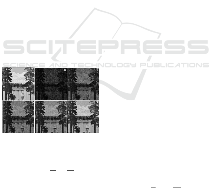
Let us illustrate the forming of sampling
representation for the standard test image “Sailboat
on the lake”, shown in Figure 4. This image was taken
from the USC-SIPI Image Database, which is often
used in image processing publications. The figure
shows several representations of a random counts of
an image having the following initial parameters:
image format - TIFF, dimensions - 512 512 pixels,
a color depth of 𝜐24 bits. First of all, the image
was converted to GIF format with the same
dimensions 512 512, but in a gray palette with a
color depth 𝜐8 bits (see Figure 4 (A)), which
allowed to reduce the overall amount of calculations.
Figures 4 B-F show samples of sizes 𝑘 = 100 000, 500
000, 1.000.000, 2.000.000 and 5,000,000, the
procedure itself was performed using the simplest
method of rejection sampling (Robert, 2004) with a
uniform auxiliary distribution 𝑔
𝑥⃗
𝑠𝑠
512
and a constant upper bound of pixel values
𝑐2
256. The choice of 𝑔
𝑥⃗
and boundary 𝑐
was due to the constraints 𝑛
2
, which in the case
of the mean 𝑚
∑
𝑛
𝑠
⁄
1 lead to the following
majorization of the distribution density of the count:
Figure 4: “Sailboat on lake” (USC-SIPI Image DB, 2021)
image representation by samples of random counts: A
original image in TIFF format, B – F representations with
the sample sizes respectively 𝑘 = 100.000, 500.000,
1.000.000, 2.000.000, and 5.000.000 counts.
𝜌𝑥⃗
|𝐼𝑥⃗ 𝜋
∑
𝑚
∑
𝑐𝑔𝑥⃗
.
(9)
As you can see, the algorithmic implementation of
the sampling method reduces to a random selection of
vectors 𝑥⃗
, uniformly distributed in the area 𝑠
𝑠 area 𝛺 with coordinates - floating-point numbers
and the inclusion of these vectors in the sample of
counts 𝑋
when performing the test (9) 𝑢
𝑛
,
where 𝑗 is the index containing the pixel 𝑥⃗
, and 𝑢
- is
the realization of a uniformly distributed over
0,𝑐 random variable (see (Robert, 2004)).
Normalization of pixels 𝑛
is not required for this
implementation.
The simplicity of forming fixed size samples of
random counts 𝑋
𝑥⃗
,…,𝑥⃗
and the universality
of the statistical description (8) of the corresponding
representation will be useful in many image
processing tasks related to classification,
identification and analysis of visual data, see
(Antsiperov, 2021). However, this approach has a
number of problems in applications related to visual
perception. This fact can be observed in the fragments
of Figure 4 - selective representations have a grainier
texture than conventional images, as a result of which
problems with the interpretation of images in the
image are possible.
At the same time, it is worth remembering that
traditional digital images are the result of rather
complex algorithms for processing original images.
TIFF image “The sailboat on the lake" in Figure 4A
is one of such images obtained by scanning a
photographic plate/film, the quality of which is
increased due to the use of post-processing methods
of the JPEG technology. Such images quality can be
obtained also with the help of digital cameras. The
above facts put us in front of solving another,
important task of improving the quality of sampling
representations for the possibility of visual perception
of graphical data. Despite the fact that this topic goes
beyond the scope of this work, leaving its solution for
future research, we will limit ourselves to the results
of the implementation of the simplest method for
smoothing noisy images, which is based on the
Parzen-Rosenblatt window method.
The smoothing method using the Parzen-
Rosenblatt window is directly related to the
nonparametric reconstruction of the probability
density function based on the kernel density
estimation (KDE) approach (Silverman, 1986). Since
in the sampling representation 𝑋
𝑥⃗
,…,𝑥⃗
the
density of the distribution of independent counts
𝜌𝑥⃗|𝐼
𝑥⃗
for our case is a multiple of the intensity
parameter 𝐼
𝑥⃗
(5), then the kernel estimate:
𝜌
𝑥
⃗
|𝑋
∑
𝐾
⃗
⃗
(10)
Image Coding by Samples of Counts as an Imitation of the Light Detection by the Retina
47

reconstructs both the density of distribution of counts
and, to the accuracy of normalization, the intensity
𝐼
𝑥⃗
(intensity form).
In (10) the kernel 𝐾
𝑥⃗
is assumed to be a non-
negative, normalized, symmetric function with a unit
second momentum on a two-dimensional plane with
coordinates 𝑥⃗𝑥
,𝑥
. In other words, the kernel is
the simplest smoothing window of unit width. The
parameter Δ0 is the smoothing parameter, it is
often also called the window width (Silverman,
1986). In our experiments, a Gaussian distribution
was used as the kernel 𝐾
𝑥⃗
𝑁
𝑥⃗
|
0
⃗
,𝐸, the
window width parameter was not used by default it
was assumed Δ1. The image dimensions were
chosen of the same size 𝑠 , 𝑠 = 512 as those of the
original image, i.e. it was assumed that the parameter
Δ of the pixel size was chosen as the scale.
Figure 5: “Sailboat on lake” (USC-SIPI Image DB, 2021)
image reconstruction using random sampling: A original
image in TIFF format, B) – F) reconstructed images by
sample sizes, respectively 𝑘 = 100.000, 500.000,
1.000.000, 2.000.000, and 5.000.000 counts.
Figure 5 shows the processed images obtained
from samples of the corresponding sizes size 𝑘 =
100.000, 500.000, 1.000.000, 2.000.000, and
5,000,000 counts (Figure 4). Separately, it is worth
noting that relatively small samples (𝑘 = 1.000.000)
generally satisfy the possibility of visual perception
of objects in the image, regardless of the presence of
blurriness and noise elements. A further increase in
the sample up to 𝑘 = 5,000,000 counts allow to get
even more useful information, such as the clarity of
the boundaries of individual objects, their relief, and
even give an assessment of other characteristics.
However, along with the increase in the sample size,
there is an increase in the time spent on its
preprocessing and recovery itself.
4 CONCLUSIONS
The paper presented a method for coding
(representing) an image by fixed size samples of
random counts. The formation of such a sampling
representation allows not only to reduce the amount
of input information but also to obtain other, not less
obvious characteristics. Particular attention is paid to
the performance of the sampling algorithm. Since
most often one must work not with the only image,
but with batches of similar images, an important
parameter is the time required to fulfil the sampling
procedure.
In the current work, attention was also paid to
estimating the time for generating samples of counts
of different sizes, which directly depends on the
number of counts specified for the formation of a
representation. With small numbers of counts, the
sampling rate for the “Sailboat on lake” image was
also small, for 𝑘 = 100,000, the time was 𝑡 = 0.71
seconds, with an increase in the sample size to 𝑘 =
1,000,000 (10 times), the time was 𝑡 = 2.68 seconds.
This difference is extremely important if we are going
to process, say, a group of 100 images, which will
take us in the best case from one minute to 4 minutes
if large sample size is selected. However, to
determine how many counts to use when coding an
image, it is necessary to operate with information
about how the image can be used for further
processing, as well as whether we can obtain a
sufficient set of properties that allow us to identify
objects and events rather accurately in the image. For
example, the representation of the image with a
sample of 𝑘 = 1.000.000 counts allow us to visually
compare the figures in the resulting coded image with
similar figures in the original one, which seems
almost impossible for a smaller sample. This allows
us to conclude that the time spent on forming a
sampling representation for images that have similar
characteristics to the “Sailboat on lake” image (size
512x512 pixels, color, with a color depth of 24 bits)
will not exceed 4 seconds, but it will take more than
1-2 seconds to form a visually interpreted image.
What about the samples of other sizes 𝑘 =
2.000.000 and 𝑘 = 5.000.000, the sampling time was
𝑡 = 10.04 seconds and 𝑡 = 20.26 seconds,
respectively. Note that such representations have
minor differences from the sample 𝑘 = 1.000.000 if
we consider the ability to visually perceive objects.
However, such samples best eliminate noise and
allow you to see smaller objects.
In general, reducing the original image with the
help of samples of counts allows not only to switch to
a new, simplified representation of the image but also
ICPRAM 2022 - 11th International Conference on Pattern Recognition Applications and Methods
48

allows to effectively perform further operations on its
processing. For the samples to be visually interpreted
even with a small number of counts, the resulting
image was restored with some degree of accuracy to
the original one by smoothing methods. The sample
size, of course, has a significant impact on the
formation time of the smoothed image, as well as on
the degree of its smoothness. This method of image
restoration allows not only to process images with
poor visual perception more accurately, but also
simplifies the task of improving the perceptual
characteristics of images with low quality and
brightness parameters. Thus, we note that the average
brightness level of the image has increased, which is
mainly due to the elimination of dark areas in the
image that remained between the recorded counts.
The time parameter spent on the implementation
of the algorithm for smoothing samples of different
sizes was also analyzed. Similarly, with the formation
of the samples themselves, the smoothing algorithm
showed the best results when working with small
samples. With the number of counts 𝑘 = 100,000,
500,000 and 1,000,000, the time was t = 0.52, 1.57
and 2.88 seconds, respectively. For large samples 𝑘 =
2.000.000 and 5.000.000 it took on average t = 5.46
and 13.24 seconds. When working with small
samples, there was an improvement in image quality
and the ability to interpret images on it. This indicates
the possibility of using small samples of counts for
image processing in the future, regardless of the
visual perception of the operator.
All the processes outlined above, aimed at
forming an ideal image, open a whole range of
possibilities in the development, improvement, and
use of various kinds of imaging devices, such as
single-photon avalanche diodes (SPAD) operating in
the mode of single photons counting.
ACKNOWLEDGEMENTS
The authors express their gratitude to the Ministry of
Science and Higher Education of Russia for the
possibility of using the Unique Science Unit
“Cryointegral” (USU #352529) designed for
simulation modelling, developed in Project No. 075-
15-2021-667.
REFERENCES
Antsiperov, V. (2019) Machine Learning Approach to the
Synthesis of Identification Procedures for Modern
Photon-Counting Sensors. Proc. of the 8th International
Conference on Pattern Recognition Applications and
Methods V. 1: ICPRAM, P. 814–821. DOI:
10.5220/0007579208140821
Antsiperov, V. (2021) Maximum Similarity Method for
Image Mining. Proceedings of the Pattern Recognition
ICPR International Workshops and Challenges, Part V.
Lecture Notes in Computer Science. V. 12665? P. 301–
313. DOI: 10.1007/978-3-030-68821-9_28.
Aull, B. F., Schuette, D. R., Young, D. J., et al. (2015) A
study of crosstalk in a 256x256 photon counting imager
based on silicon Geiger–mode avalanche photodiodes.
IEEE Sens. J., V. 15(4), P. 2123-2132.
Barber, D. (2012) Bayesian Reasoning and Machine
Learning. Cambridge Univ. Press. Cambridge.
Bertero, M., Boccacci P., et al. (2009) Image deblurring
with Poisson data: from cells to galaxies. Inverse
Problems, V. 25(12), IOP Publishing, P. 123006. DOI:
10.1088/0266-5611/25/12/123006.
Dutton, N. A. W., Gyongy, I., Parmesan, L., et al. (2016).
A SPAD–based QVGA image sensor for single–photon
counting and quanta imaging. IEEE Trans. Electron
Devices V. 63(1), P. 189-196.
Fossum, E. R., Teranishi, N., et al. (2017) Photon-Counting
Image Sensors. MDPI. DOI: 10.3390/books978-3-
03842-375-1.
Fox, M. (2006) Quantum Optics: An Introduction. U. Press,
New York. DOI: 10.1063/1.2784691.
Gabriel, C. G., Perrinet, L., et al. (2015) Biologically
Inspired Computer Vision: Fundamentals and
Applications. Wiley-VCH, Weinheim.
Gallager, R. (2013) Stochastic Processes: Theory for
Applications. Cambridge University Press, Cambridge.
DOI: 10.1017/CBO9781139626514.
Gonzalez, R. C., Woods, R. E. (2007) Digital Image
Processing 3
d
edition. Prentice Hall, Inc.
Goodman, J. W. (2015) Statistical Optics 2
nd
edition. Wiley,
New York.
Holst, G.C. (2011) CMOS/CCD sensors and camera
systems. SPIE Press. Bellingham. DOI:
10.1117/3.2524677
Koch, K., McLean, J., et al. (2006) How much the eye tells
the brain? Current biology: CB, V.16(14): 1428–1434.
DOI: 10.1016/j.cub.2006.05.056.
Morimoto, K., Ardelean, A., et al. (2020) Megapixel time-
gated SPAD image sensor for 2D and 3D imaging
applications. Optica V. 7, P. 346-354. DOI:
10.1364/OPTICA.386574.
Pal, N.R., Pal, S.K. (1991) Image model, poisson
distribution and object extraction. International Journal
of Pattern Recognition and Artificial Intelligence, V.
5(3), P. 459–483. DOI: 10.1142/S0218001491000260.
Robbins, M. (2011) Electron-Multiplying Charge Coupled
Devices-EMCCDs. In Single-Photon Imaging, Seitz, P.
and Theuwissen, A. J. P. (eds.). Springer, Berlin, P.
103-121.
Robert, C.P., Casella G. (2004) Monte Carlo Statistical
Methods (2-nd edition). New York: Springer-Verlag.
DOI: 10.1007/978-1-4757-4145-2
Rodieck, R. W. (1998) The First Steps in Seeing.
Sunderland, MA. Sinauer.
Image Coding by Samples of Counts as an Imitation of the Light Detection by the Retina
49

Streit, R. L. (2010) Poisson Point Processes. Imaging,
Tracking and Sensing. Springer, New York.
Silverman, B.W. (1986) Density Estimation for Statistics
and Data Analysis. Chapman & Hall/CRC/ London.
DOI: 10.1007/978-1-4899-3324-9.
USC-SIPI Image DB [USC-SIPI Image Database]. last
accessed 2021/09/21.
ICPRAM 2022 - 11th International Conference on Pattern Recognition Applications and Methods
50
