Image-set based Classiﬁcation using Multiple Pseudo-whitened Mutual

Subspace Method

Osamu Yamaguchi

1,2

and Kazuhiro Fukui

Department of Computer Science, Graduate School of Systems and Information Engineering, University of Tsukuba, Japan

Corporate Research and Development Center, Toshiba Corporation, Japan

Keywords:

Image-set based Classiﬁcation, Whitening Transformation, Multiple Pseudo-Whitened Mutual Subspace

Method, Ensemble Method, CNN Features.

Abstract:

This paper proposes a new image-set-based classiﬁcation method, called Multiple Pseudo-Whitened Mutual

Subspace Method (MPWMSM), constructed under multiple pseudo-whitening. Further, it proposes to com-

bine this method with Convolutional Neural Network (CNN) features to perform higher discriminative per-

formance. MPWMSM is a type of subspace representation-based method like the mutual subspace method

(MSM). In these methods, an image set is compactly represented by a subspace in high dimensional vector

space, and the similarity between two image sets is calculated by using the canonical angles between two cor-

responding class subspaces. The key idea of MPWMSM is twofold. The ﬁrst is to conduct multiple different

whitening transformations of class subspaces in parallel as a natural extension of the whitened mutual subspace

method (WMSM). The second is to discard a part of a sum space of class subspaces in forming the whiten-

ing transformation to increase the classiﬁcation ability and the robustness against noise. We demonstrate the

effectiveness of our method on tasks of 3D object classiﬁcation using multi-view images and hand-gesture

recognition and further verify the validity of the combination with CNN features through the Youtube Face

dataset (YTF) recognition experiment.

1 INTRODUCTION

For the past few decades, many image set-based

techniques have been proposed (Zhao et al., 2019).

These techniques have been applied to face recog-

nition (Taskiran et al., 2020), 3D object recognition

(Wang et al., 2018a), and gesture recognition (Wang

et al., 2018b), and are an essential technology in com-

puter vision.

In this paper, we propose a new image-set-based

classiﬁcation, called Multiple Pseudo-Whitened Mu-

tual Subspace Method (MPWMSM), which is con-

structed under multiple pseudo-whitening trans-

formations. MPWMSM is a type of subspace

representation-based method like the mutual subspace

method (MSM) (Maeda and Watanabe, 1985; Ya-

maguchi et al., 1998) . In subspace-based meth-

ods, image set is compactly represented as a sub-

space, features are extracted by projection from the

subspace representation to a discriminative space,

and classiﬁcation is performed using the angle be-

tween the subspaces as a similarity. In order to

improve the discriminative performance, the Con-

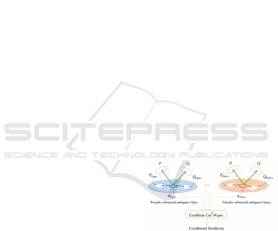
Figure 1: Overview of proposed Multiple Pseudo-Whitened

Mutual Subspace Method.

strained Mutual Subspace Method (CMSM) (Fukui

and Yamaguchi, 2003), the Multiple Constraint Mu-

tual Subspace Method (MCMSM) (Nishiyama et al.,

2005), and the Whitened Mutual Subspace Method

(WMSM) (Kawahara et al., 2007) have been proposed

as methods to perform feature extraction before the

mutual subspace method.

Fig. 1 shows the overview of the proposed MP-

WMSM. As the discriminant space in the proposed

method, we adapt the whitening transformation with

296

Yamaguchi, O. and Fukui, K.

Image-set based Classiﬁcation using Multiple Pseudo-whitened Mutual Subspace Method.

DOI: 10.5220/0010836500003122

In Proceedings of the 11th International Conference on Pattern Recognition Applications and Methods (ICPRAM 2022), pages 296-306

ISBN: 978-989-758-549-4; ISSN: 2184-4313

a modiﬁed eigenvalue weighting, which is called the

pseudo-whitening transformation (O

in Fig. 1).

The components of whitening transformation with

larger index are heavily weighted by the scaling fac-

tors that are highly sensitive to noise in the training

data. In practice, disturbances due to noise can be ob-

served and the classiﬁcation using these components

causes performance degradation. Discarding a part of

a sum space of class subspaces in forming the whiten-

ing transformation increases the classiﬁcation ability

and the robustness against noise. Next, the two sub-

spaces, P and Q, to be compared are transformed by

multiple projection calculation using O

indepen-

dently as shown in Fig. 1. Each projection O

can

be used with a transformation consisting of a subset

of the training data. Lastly, the similarity between the

transformed subspaces is calculated respectively, and

the ﬁnal similarity is obtained by integrating multiple

similarities. The combination of multiple feature ex-

tractions can achieve even higher accuracy due to the

effect of ensemble learning with reducing overtrain-

ing and small variances.

Furthermore, in recent years, Convolutional Neu-

ral Network (CNN) features have shown high ef-

fectiveness in discriminative performance in various

ﬁelds (Razavian et al., 2014; Azizpour et al., 2016).

Several works have been already published showing

the performance improvement by combining the mu-

tual subspace method with CNN features (Sogi et al.,

2018; Sakai et al., 2019). In our study, we use off-the-

shelf CNN features without retraining Deep Convolu-

tional Neural Networks (DCNNs) to reduce the train-

ing cost for the target domain. While we could take

advantage of the training data to improve the CNN

features with further ﬁne-tuning, it is necessary to ﬁrst

ensure that the subspace-based feature extraction for

image set works well.

The contributions of this paper include the follow-

ing:

• To improve the noise tolerance to the whitening

transformation, we classiﬁed the discriminative

subspace into three categories based on the anal-

ysis of the eigenspectrum and studied the pseudo-

whitening transformation.

• The MPWMSM method, which combines multi-

ple feature extraction based on ensemble learn-

ing, is used to improve performance using sub-

space representations of off-the-shelf CNN fea-

tures without retraining DCNNs.

• We applied the proposed method to several ap-

plications and conﬁrmed its effectiveness. As a

result, we achieved the state-of-the-arts accuracy

for YouTube Faces dataset (YTF) using the latest

deep learning features.

The paper is organized as follows. First, we out-

line the conventional algorithms of MSM, CMSM,

and WMSM in section 2. In order to propose a new

discriminant space, we review each method in terms

of how it introduces the discriminant space. Sec-

tion 3 describes an extension of Whitening transfor-

mation by modiﬁcation of eigenvalue weighting and

an integrated similarity calculation of multiple fea-

ture extraction methods similar to ensemble learning.

In section 4, we compare the performance on 3D ob-

ject recognition, gesture recognition, and video-based

face recognition using a dataset for image-set based

recognition. Finally we conclude our paper by sum-

marizing the paper.

2 RELATED WORK ON

SUBSPACE-BASED METHODS

In this section, we describe the subspace-based

matching algorithms (Yamaguchi et al., 1998) and

constrained mutual subspace method (Fukui and Ya-

maguchi, 2003) and the whitened mutual subspace

method (Kawahara et al., 2007). Finally, we describe

the problem of WMSM and analyze it from the view

of eigenspectrum. Then, we make a comparison of

the transformation in CMSM and WMSM.

2.1 Mutual Subspace Method

Mutual Subspace Method (MSM) (Maeda and Watan-

abe, 1985) is a method that approximates the entire

pattern variation by a subspace and measures the sim-

ilarity by the angle between the subspaces. This is an

extension of the Subspace Method (Oja, 1983), which

performs identiﬁcation based on the minimum angle

between two subspaces, the input subspace and the

reference subspace.

The identiﬁcation based on this minimum angle

uses the concept of a canonical angle and is gener-

alized by multiple canonical angles. Between the m-

dimensional subspace P and the n-dimensional sub-

space Q, n canonical angles (n < m) can be deﬁned,

and the ﬁrst canonical angle θ

is the minimum angle

between the two subspaces.

The second canonical angle θ

is the minimum an-

gle measured in the direction orthogonal to the mini-

mum canonical angle θ

. Similarly, the following n

canonical angles θ

(i = 1 ... n) can be obtained se-

quentially. The minimum canonical angle is deter-

mined by the angle between the two subspaces, θ

, in

the equation (1). Similarity S between patterns is then

used for classiﬁcation (Yamaguchi et al., 1998).

Image-set based Classiﬁcation using Multiple Pseudo-whitened Mutual Subspace Method

297

S = cos

(1)

The cos

is the maximum eigenvalue λ

max

of the

following matrix X.

Xa = λa (2)

X = (x

) (m,n = 1 .. .N

) (3)

∑

l=1

(ψ

,φ

)(φ

,ψ

) (4)

where ψ

,φ

are the m, lth orthonormal basis vectors

in the subspaces P and Q, where (ψ

,φ

) is the inner

product of ψ

and φ

, and N

is the number of basis

vectors in the subspace.

The canonical angles between the two subspaces

can be obtained plurals as described. In practice, we

consider the value of the mean of the canonical an-

gles,

S[t] =

∑

i=1

cos

, (5)

as the similarity between two subspaces. The value

S[t] reﬂects the structural similarity between two sub-

spaces.

2.2 Constrained Mutual Subspace

Method and Generalized

Differential Subspace

In the previous section, we explained how MSM clas-

siﬁes a set of feature vectors in the original vector

space. However, the original space is not exactly fa-

vorable for discriminating the subspaces, and it is de-

sirable to embed each subspace in a more discrimina-

tive space.

To improve the discrimination performance, the

input subspace P and the reference subspace Q are

projected onto the constrained subspace C consisting

of the components effective for discrimination, and

the canonical angles are measured for the projections

and Q

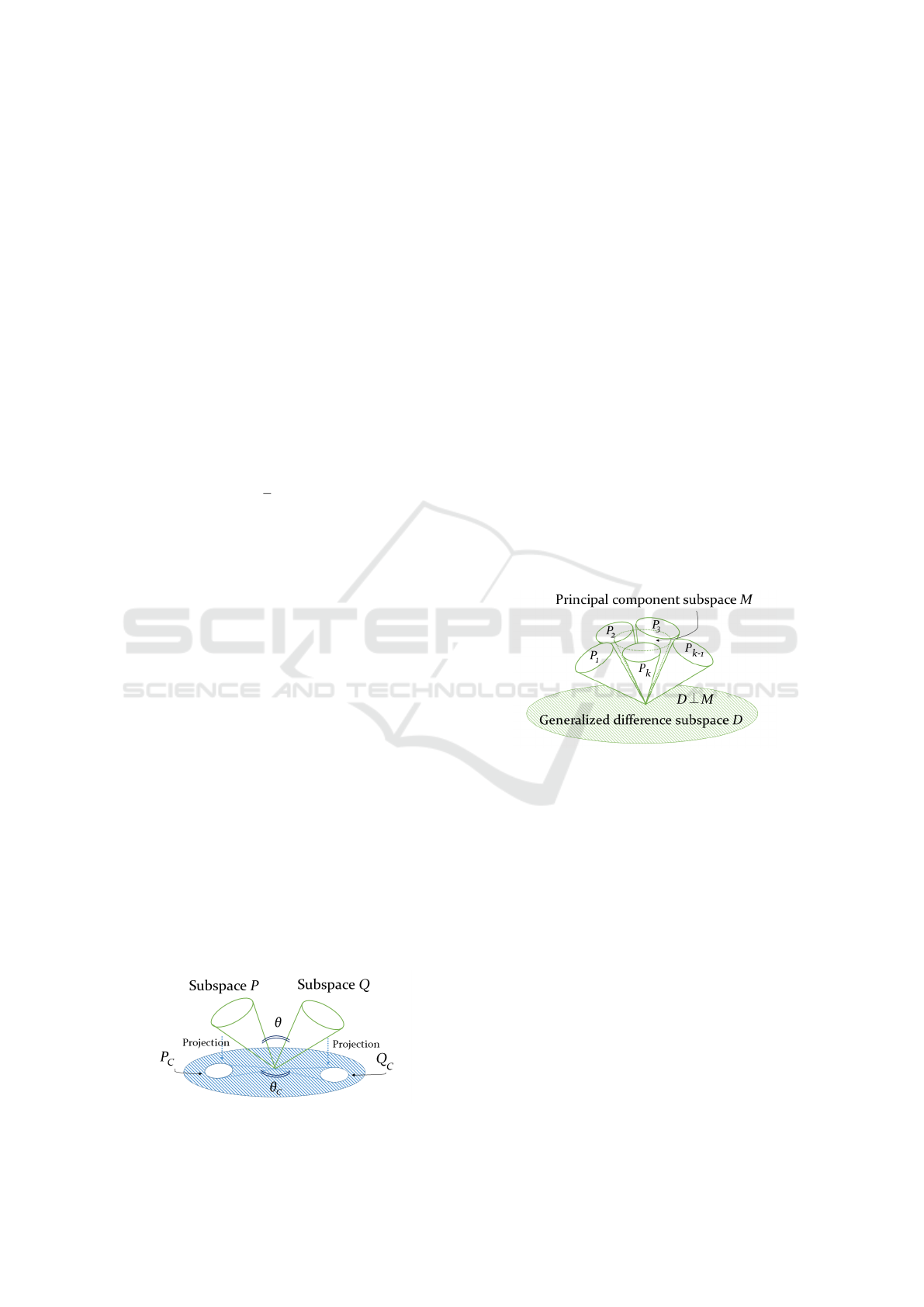
, as shown in Figure 2. This method adds

the projection onto the constrained subspace to the

mutual subspace method and is called Constrained

Mutual Subspace Method (CMSM) (Fukui and Yam-

aguchi, 2003).

Figure 2: Concept of CMSM.

Futhermore, there is also a method that uses the

generalized differential subspace (Fukui and Maki,

2015). The generalized difference subspace D is

obtained by ﬁrst calculating the sum matrix G =

∑

i=1

, where P

are the projection matrices of R n-

dimensional reference subspaces. The basis vectors

are then obtained by performing the following eigen-

value decomposition:

Gd = λd (6)

where the eigenvectors d

correspond to the i-th eigen-

value λ

in descending order. Finally, only the N

eigenvectors with smallest eigenvalue are kept as the

basis vectors for D. Such dimension is set experimen-

tally.

As shown in Fig. 3, the generalized difference

subspace D is obtained by removing the principal

component space M, which doesn’t contain useful in-

formation for discrimination, from the sum space of

all class subspaces. Geometrically, by removing the

space M, the angle between each class subspace pro-

jected to the generalized difference subspace is ex-

panded.

Figure 3: Concept of generalized difference subspace.

2.3 Whitened Mutual Subspace Method

This section describes the whitening transformation

of a set of subspaces as a process to emphasize the

differences between the subspaces representing each

class. The whitening transformation for a set of sub-

spaces is formulated as an approximate solution to

the minimum value problem of the objective function,

which becomes smaller as the angle between the sub-

spaces increases. Let the set of d-dimensional sub-

spaces of each class be V

,. ..,V

and the d canonical

angles of V

and V

be θ

(1)

i j

,. ..,θ

(d)

i j

. Then, the follow-

ing equation holds for the sum of the squares of the

cosines of the canonical angles.

∑

1≤<i≤R

∑

k=1

cos

(k)

i j

= C

, (7)

ICPRAM 2022 - 11th International Conference on Pattern Recognition Applications and Methods

298

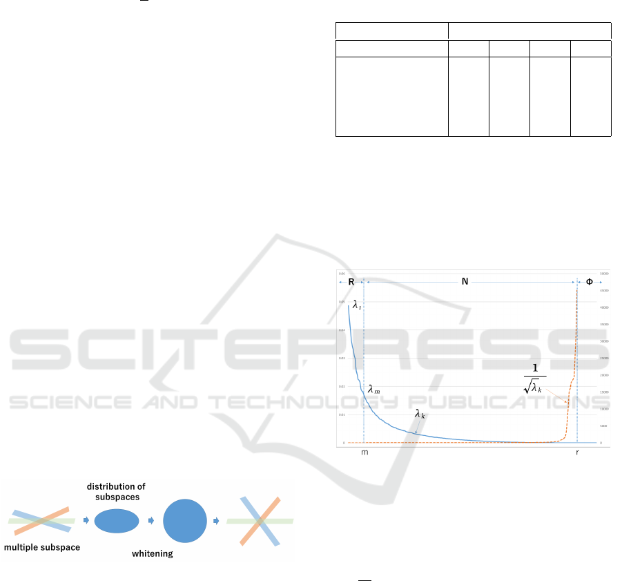
where C

are positive constants and σ

is the vari-

ance of the eigenvalues of the autocorrelation matrix

G of the set of subspaces deﬁned below:

G =

∑

i=1

. (8)

is a projection matrix (1 ≤i ≤ R) deﬁned in the

basis ψ

,. ..,ψ

of V

as following equation,

∑

k=1

. (9)

From this equation, we can see that the smaller the

variance of the eigenvalues of the matrix G, the wider

is the angle between the subspaces that generated G.

Therefore, the variance of the eigenvalues of the au-

tocorrelation matrix G is minimized by the whitening

transformation W , which sets all eigenvalues to 1, as

deﬁned below.

G = BΛB

. (10)

W = Λ

−1/2

, (11)

where Λ is the diagonal matrix of the eigenvalues of

the autocorrelation matrix G, and B is the matrix of its

eigenvectors arranged vertically.

Figure 4 shows how the whitening transforma-

tion expands the angles between the subspaces. Since

the whitening transformation spreads the angles uni-

formly, the pairs of subspaces with smaller angles be-

tween them will expand more. Therefore, when the

whitening transformation is applied to the subspace

of a certain class, the angle expands in the subspace

of similar classes, emphasizing the difference.

Figure 4: The ellipse and the circle in the center of the ﬁgure

represent the distribution of subspaces. Whitening makes

the distribution uniform.

2.4 The Problems of Previous Methods

2.4.1 Analysis in View of the Eigenspectrum

In order to prevent the reference subspaces of each

class from being similar to each other, the whitened

mutual subspace method linearly transforms the refer-

ence subspaces into a feature space where the angles

between the reference subspaces are apart, thereby

improving the discrimination accuracy.

However, we have observed in the literature

(Fukui and Yamaguchi, 2006) an interesting result for

the ETH-80 dataset (Leibe and Schiele, 2003).

Table 1: Results for 3D object recognition in (Fukui and

Yamaguchi, 2006).

Accuracy (%)

S[1] S[2] S[3] S[4]

MSM 72.7 73.7 76.3 74.3

CMSM-215 75.7 81.3 76.3 73.7

CMSM-200 73.3 81.0 79.3 77.7

CMSM-190 71.0 73.0 73.0 75.7

WMSM(OMSM) 51.3 54.0 56.0 54.0

As we can see in Table. 1, despite the whitening

transformation, WMSM perform worse than MSM.

This means that feature extraction has lost its meaning

despite the use of discriminant transformations with

the subspace. To improve this performance degra-

dation, we revise the feature extraction by whitening

transformation.

Figure 5: A real distribution of eigenvalues in descending

order (solid line) and the weights of whitening transforma-

tion (dashed line). m denotes split point between Reliable

subspace (R) and Noise subspace (N). r denotes split point

between Noise subspace and Null subspace(Φ).

Fig. 5 shows the distribution of eigenvalues of

G (Eq. (6) ) in descending order and the weights

(1/

) of whitening transformation. The compo-

nents of whitening transformation of larger index are

heavily weighted by the scaling factors.

The discussion of the eigenspectrum has been dis-

cussed in (Jiang et al., 2008). This paper points

out that noise turbulence and poor estimates of small

eigenvalues due to the ﬁnite number of training sam-

ples are the culprits. Due to the limited number of

training samples, the eigenvalues for a dimension can

be so small that they do not represent the true vari-

ance of that dimension well. This may result in se-

vere problems if their inverses are used as the weight

for the whitening transformation.

Image-set based Classiﬁcation using Multiple Pseudo-whitened Mutual Subspace Method

299

We estimate the eigenspectrum using the equation

in (Jiang et al., 2008). The two parameters α and β,

and the estimating equation are deﬁned by Eq. (12).

(13) and (14).

α =

(m −1)

−λ

, (12)

β =

mλ

−λ

, (13)

k + β

, (14)

where λ

is the maximum eigenvalue, λ

is the eigen-

value of the split points m, and

is the estimated

eigenvalue. The subspaces are divided into three cat-

egories, i.e., Reliable subspace (R), Noise subspace

(N), and Null subspace (φ) (Jiang et al., 2008). The

split point indicates the index m that separates the re-

liable subspace (R) from the noise subspace (N), as

shown in Fig. 5.

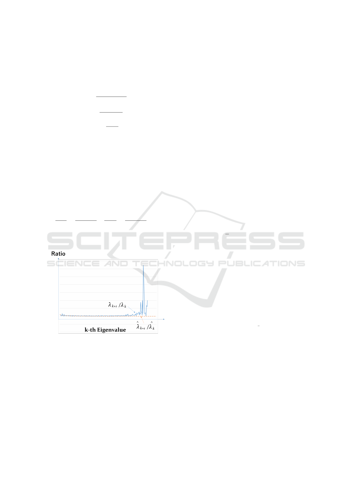
We introduce the eigenvalue ratios to observe how

much they differ from the estimated variance,

k+1

k + 1 + β

k + β

k + 1 + β

. (15)

Eq. (15) is a monotonically decreasing function

and it calculates the ratio between

and

k+1

Figure 6: The comparison of the real eigenvalue ratio (solid

line) and estimated eigenvalue ratio (dashed line) . The os-

cillations arises in the components with large index.

Figure 6 plots the real and estimated eigenvalue

ratio values. It is desirable that the eigenvalue ratios

always decay, even in the high-dimensional part of

the whitening transformation. However, in the large

index eigenvalue part, many of them deviate from the

estimated values. This disturbance leads to large os-

cillations in the inverse eigenspectrum. The compo-

nents with large index k are strongly sensitive to noise

due to training data, leading to poor recognition per-

formance on test data.

In the next section, the discussion will focus on

controlling the magnitude of the eigenvalues of the

autocorrelation matrix of the basis vectors used to

compute the feature extraction.

2.4.2 Comparison between Projection to

Constrained Subspaces and Whitening

Transformation

The constrained mutual subspace method (CMSM)

and the whitened mutual subspace method (WMSM)

are both methods to obtain the transformation matrix

based on the autocorrelation matrix G of the projec-

tion matrix generated from the reference subspace.

The projection matrix P

is deﬁned by Eq. (16), where

i j

is the j-th orthonormal basis vector of the refer-

ence subspace of the i-th category and N

is the num-

ber of basis vectors of the reference subspace.

In the CMSM, the constrained subspace O

CMSM

deﬁned using the projection matrix of each category

by Eq. (18).

∑

j=1

i j

, (16)

G =

+ P

+ ···+ P

), (17)

CMSM

∑

k=1

, (18)

where R is the number of reference subspaces, φ

the kth eigenvector selected from the smaller eigen-

values of the matrix G, and N

is the number of eigen-

vectors of the matrix G.

On the other hand, in the whitening mutual sub-

space method, the transformation matrix for whiten-

ing the reference subspaces O

W MSM

is deﬁned by the

Eq. (19).

W MSM

= Λ

−

. (19)

As before, B is the matrix of eigenvectors of G, and

Λ represents the diagonal matrix of the eigenvalues of

G. O

CMSM

is represented using the following C

CMSM

= C

, (20)

= diag(0,0,0,.. .,0, 1, 1,1,1). (21)

In this case, C

is the diagonal matrix of rank N

This weight distribution is shown in Figure 7. The

graph shows the weights of the eigenvectors in each

method. In CMSM, only the vectors after a particu-

lar dimension are used, and the weight is 1.0 in each

case. In the WMSM, on the other hand, the weights

ICPRAM 2022 - 11th International Conference on Pattern Recognition Applications and Methods

300

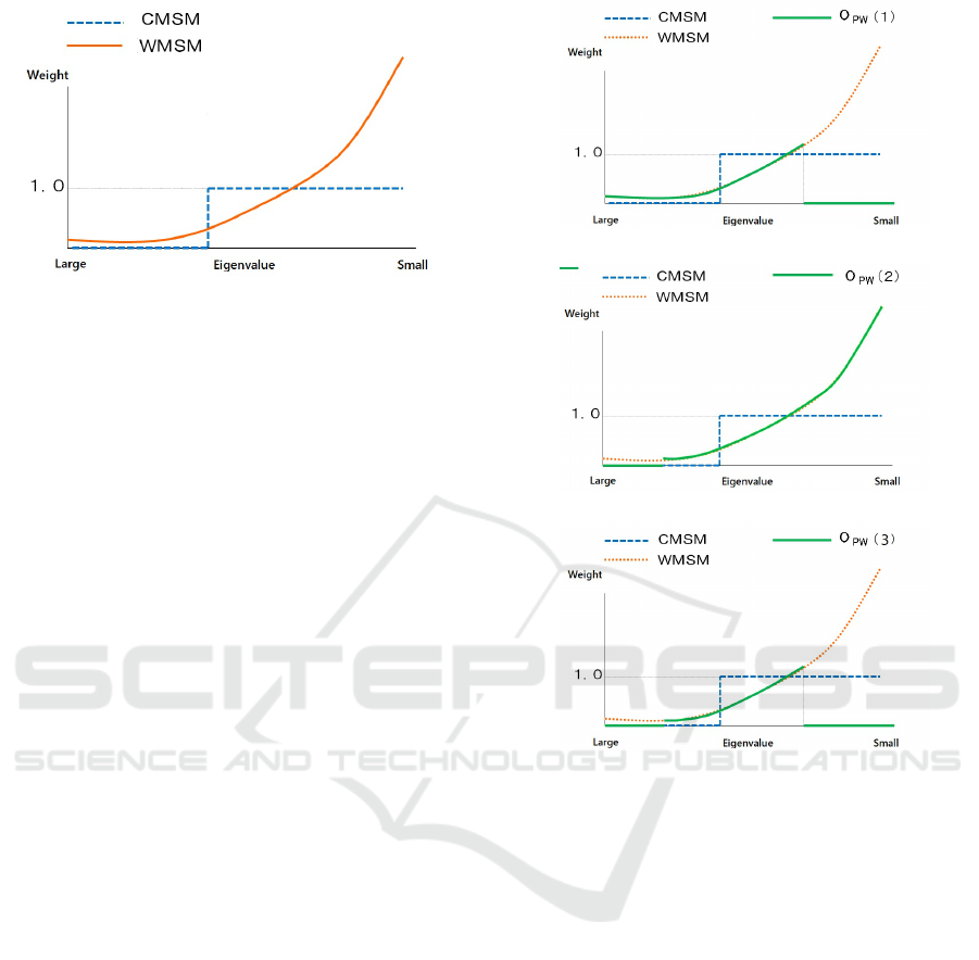
Figure 7: Weighting of Constraint subspace and Whitening

transformation.

are the square root of the reciprocals of the eigenval-

ues, and thus the weights become larger for higher

dimensions. This ﬁgure also shows that eigenvectors

of lower dimensions, which are discarded in CMSM,

are given small values in WMSM, while eigenvec-

tors of higher dimensions are given large weights. In

the WMSM, the components extracted by the high-

dimensional eigenvectors are given more importance,

which may cause cases of high similarity between

classes and may lead to a decrease in performance.

This does not occur in the CMSM due to introducing

constant weights.

3 PROPOSED METHOD

In this section, we describe our method, MPWMSM.

We introduce the pseudo-whitening transformation.

After that, we describe the proposed method which

combines multiple feature extraction.

3.1 Introduction of Pseudo-whitening

Transformation

As in the case of the CMSM, we propose to select

the features to be extracted by setting the weights of

some basis vector components to zero, which is like a

combination of WMSM and CMSM.

Figure 8 shows the weighting of the whitening

transformation with different parts set to zero. In Fig.

8(a), the high-dimensional part is set to 0, and in Fig.

8(b), the low-dimensional part is set to 0. Further-

more, in Fig. 8(c), both parts are set to 0 simultane-

ously.

Such weighting has been already discussed

in terms of eigenspectrum regularization models

(ERMs) (Jiang et al., 2008; Tan et al., 2018). These

methods focus on weighting using the full rank. The

CMSM is considered to be divided into two sub-

(a) Eliminate high-dimensional parts

(b) Eliminate low-dimensional parts

Figure 8: Variation of changing weights of whitening trans-

formations.

spaces, principal component subspace and general-

ized difference subspace as shown in Figure 3, and the

split points are deﬁned for the binary weights shown

in Figure 7. In our method, we divide the subspace

into three categorized subspaces: principal compo-

nent subspace, reliable difference subspace, and noise

subspace, as shown in Figure 9. The discriminative

space is deﬁned by their combination.

To achieve this, we ﬁlter some of the diagonal

components of the matrix Λ, such as some of the

small eigenvalues or some of the large eigenvalues,

setting them to 0, and make changes to it as a pseudo-

whitening matrix O

Then, by replacing the whitening matrix O

W MSM

of the whitening mutual subspace method with the

pseudo-whitening matrix O

, it is expected to im-

prove the results for the cases where the WMSM does

not outperform MSM.

The pseudo-whitening matrix O

is deﬁned by

Image-set based Classiﬁcation using Multiple Pseudo-whitened Mutual Subspace Method

301

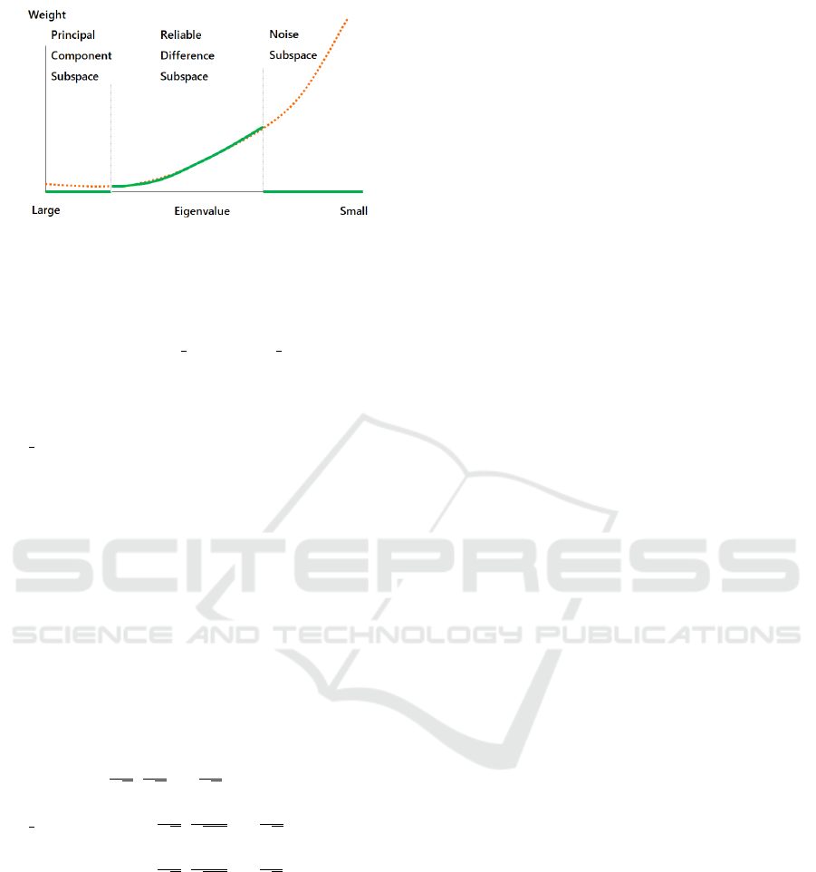
Figure 9: Subspaces divided into three categorized parts in

our method. As for the weights of Principal Component

Subspace and Noise Subspace, we control them by setting

them to zero.

the Equation (22).

= C

−

= Λ

−

. (22)

Here, B is a matrix of eigenvectors, Λ is a diag-

onal matrix of eigenvalues, and C

is a diagonal ma-

trix with 0 and 1 elements given by the equation (23).

−

is given by the equation (24), where j and k de-

note the dimensions that deﬁne the range to be set to

0. Several of the eigenvalues of Λ are replaced by ze-

ros. We can replace some eigenvalues with 0 using

various C











diag(1,.. . ,1,. ..,1, 0,.. . ,0) .. . (a)

diag(0,.. . ,0,1, ..., 1,.. . ,1) .. . (b)

diag(0,.. . ,0,1, ..., 1,0,. . .,0) . .. (c)

j k

(23)

−











diag(

√

,...,

√

,0,...,0) . . . (a)

diag(0,...,0,

√

,...,

√

) . . . (b)

diag(0,...,0,

√

,...,

√

,0,...,0) . . . (c)

(24)

Therefore, the Mutual Subspace Method using

the pseudo-whitening transformation O

is denoted

as the Pseudo-Whitened Mutual Subspace Method

(PWMSM).

3.2 Multiple Pseudo-whitened Mutual

Subspace Method

This section presents the Multiple Whitened Mu-

tual Subspace Method (MWMSM) and the Multi-

ple Pseudo-Whitened Mutual Subspace Method (MP-

WMSM) in which we applied ensemble learning to

the Whitened Mutual Subspace Method. This ap-

proach follows (Nishiyama et al., 2005)

To extract effective features for set-based image

recognition, we transform the input subspace and the

reference subspace into multiple feature transforma-

tion. In the experiment we obtained high performance

compared with projecting onto a single transforma-

tion. To generate multiple transformations, we apply

the framework provided by ensemble learning.

Figure 1 in Section 1 shows process diagram of

Multiple Pseudo-Whitened Mutual Subspace Method

(MPWMSM). The multiple pseudo-whitening trans-

formations are represented by the projection matrix

in Eq. (22).

To generate multiple feature extractor in this pa-

per, we use the concept of Bagging (Breiman, 1996),

which is based on an ensemble learning algorithm.

Multiple classiﬁers are constructed using random

sampling in Bagging. To apply this framework to gen-

erating feature extractor, we randomly select L

(< L)

subspaces from L class subspaces. Each projection

subspace is generated independently using selected

training subspaces.

In summary, we generate M constraint subspaces

by the following steps:

1. Select L

class subspaces randomly without re-

placement.

2. Generate a projection subspace using selected L

class subspaces in Eq. (22).

3. Until M projection subspaces are generated, go to

step 1.

To combine similarities obtained on each projec-

tion subspace, we deﬁne the combined similarity S

as follows:

∑

i=1

, (25)

where M is the number of the pseudo-whitening trans-

formations; α

is the i-th coefﬁcient of O

; S

the similarity between P

and Q

projected onto

4 EXPERIMENTS

In this section, we will present the experimental eval-

uation of our proposed method. We performed mainly

three experiments, to be explained in the following

subsections.

ICPRAM 2022 - 11th International Conference on Pattern Recognition Applications and Methods

302

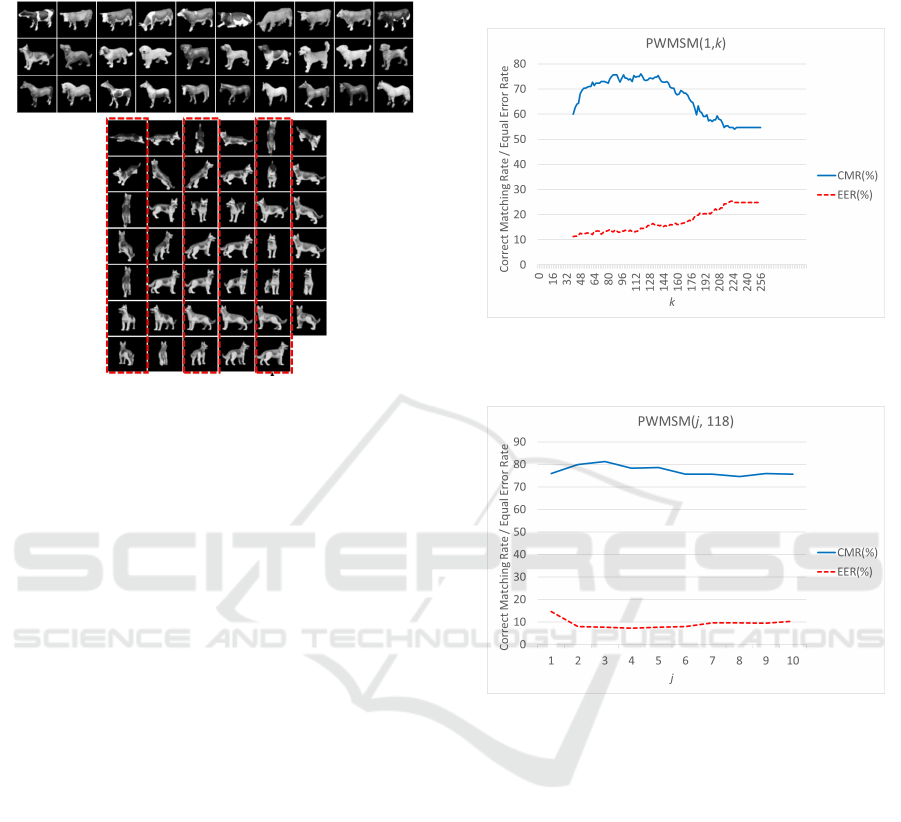
4.1 3D Object Recognition (ETH-80)

Figure 10: Object Recognition experiment using ETH-80.

Top: Selected 30 classes for similar shape classiﬁcation

test. Bottom: All patterns of dog1 (the dotted columns are

the training images).

We carried out our experiments using the ETH-

80 dataset, which consists of 3D models taken from

multiple viewpoints, as shown in Fig. 10. From this

database, 30 models with similar shapes are extracted.

The experimental conditions for these models are in

accordance with the literature (Fukui and Yamaguchi,

2007). Therefore, CNN features are not used in this

experiment for comparison with conventional proto-

cols.

For each model, a set of images is taken from 41

viewpoints for each object, as shown in Figure 10.

The viewpoints are the same for all models. Of these,

the odd-numbered images (21) are used as the class

subspace, while the even-numbered images (20) are

used as the evaluation data. In other words, the learn-

ing perspective is different from the evaluation per-

spective. For the evaluation data, we took 10 images

from i to i + 9 out of the 20 images to make one

data set, and prepared a total of 10 evaluation sets by

changing the starting frame i from 1 to 10. Therefore,

the total number of trials is 300 (=10×30).

The original image was converted to a

monochrome image of 16 × 16 pixels for the

evaluation. Thus, the dimensionality of the data

is 256. The dimensionality of the input subspace

and the reference subspace of each class was set to

7, and the dimensionality of the subspace used for

training (N

) was set to 20. For direct comparison

with WMSM, no multiplication is applied, and the

evaluation is performed as M = 1 and α

= 1.0 in Eq.

(25).

Here, PWMSM ( j, k) represents the case where

the j-th to k-th elements in Eq. (23) are set to 1.

Therefore, PWMSM(1, 256) is the same as WMSM.

Figure 11: The correct matching rate and the equal error

rate of PWMSM(1, k) for different dimension of k. O

eliminated part of higher dimension.

Figure 12: The correct matching rate and the equal error

rate of PWMSM( j, 118) for different dimension of j. O

is eliminated both part of higher and lower dimension.

Figure 11 shows the correct matching rate and the

equal error rate of PWMSM(1, k) for different dimen-

sion of k. The results were obtained by varying from

the 40th dimension to the 256th dimension sequen-

tially. This refers to classiﬁcation accuracy improved

to 76.0% compared to 54.6% for the original whiten-

ing transformation.

The result of ﬁxing the 118th dimension at the

maximum value and changing the elements of C

Eq. (23) from the low-dimensional part to 0, i.e.

PWMSM( j, 118) is shown in Fig. 12. In this case, the

results further improved to 81.4%. When compared to

S[1] in Table 2, it is found to exceed the performance

of other linear feature extraction schemes.

Our best performance of PWMSM was achieved

when using 3 - 100 dimensions, resulting in 83.3% in

classiﬁcation accuracy. This is the best performance

among the subspace-based methods we compared.

Image-set based Classiﬁcation using Multiple Pseudo-whitened Mutual Subspace Method

303

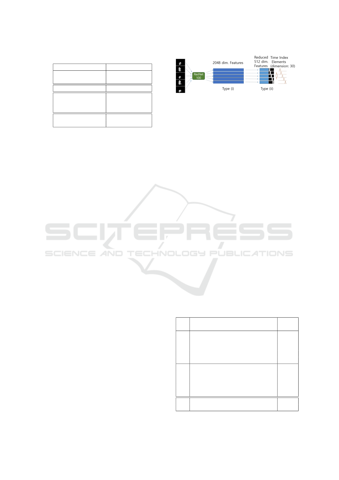
Table 2: Results for 3D object recognition.

Acc. (%) by S[1]

MSM 72.7

CMSM-215 75.7

WMSM 54.6

PWMSM (1, 118) 76.0

PWMSM (3, 118) 81.4

PWMSM (3, 100) 83.3

MWMSM 11.0

MPWMSM (3, 104) 84.0

Table 2 summarizes the results and compares the

proposed method with the results from a conventional

linear feature extraction system.

In addition, feature selection performed by the

PWMSM can embed the data in a smaller dimension

than the original data dimension. We believe this is

of great practical signiﬁcance, as it improves the stor-

age efﬁciency of the reference subspace and reduces

computational cost.

Furthermore, to perform the multiple version of

proposed methods, the MWMSM and MPWMSM,

the training data is divided into three parts, and the

discriminant transformation is created from 10 sam-

ples of each part. We conﬁrmed that the performance

could be further improved by the multiple pseudo-

whitening transformations, while it gets worse by the

multiple whitening transformations.

4.1.1 Hand Gesture Recognition (IPN Hand)

Hand gesture recognition (HGR) is an essential func-

tion of human-computer interaction, which has a wide

range of applications. IPN Hand (Benitez-Garcia

et al., 2021) is a video dataset for real-time hand ges-

ture recognition. The gestures in this dataset focused

on interaction with touchless screens, including 13

categories. In the 50 subjects, there are 16 females

and 34 males. The dataset was collected from about

30 diverse scenes, with real-world variation in back-

ground and illumination.

We tried the Isolated HGR task, which is eval-

uated as the conventional classiﬁcation metric. The

data split the data by subject into training (74%) and

testing (26%) sets, resulting in 148 training and 52

testing videos. The numbers of gesture instances in

training and testing splits are 3,117 and 1,101, respec-

tively. In this experiment, we use the RGB-seg used

in literature (Benitez-Garcia et al., 2021). Semantic

segmentation masks were provided as annotated data

and we segmented the RGB images using the masks.

The images are processed by the public pre-trained

ResNet-100 model by ImageNet train, and 2048 di-

Figure 13: Frame Features for HGR. Type (i) is a 2048 di-

mensional feature extracted from DCNNs for each frame;

Type (ii) uses features reduced to 512 dimensions from the

original DCNNs features by PCA and add a time index ele-

ment to represent the time transition.

mensional features are extracted from the C5 layer.

Note that the training data was not used to train the

DCNNs. We use the training data only for subspace-

based feature extraction.

Each gesture instance’s start and end frame index

in the video was manually labeled, providing enough

information to train for forming the subspace. The

video sequences are segmented into isolated gesture

samples based on the beginning and ending frames

manually annotated. We use classiﬁcation accuracy to

evaluate our method, which is the percent of correctly

labeled examples.

Table 3 shows the results for IPN Hand classiﬁ-

cation. We tried two types of features as shown in

Fig. 13. Type (i) is a 2048 dimensional feature ex-

tracted from DCNNs for each frame; Type (ii) uses

features reduced to 512 dimensions from the origi-

nal DCNNs features by PCA. Moreover, we add a 30-

dimensional time index element to represent the time

transition. For the time index, we let the normal distri-

bution move along the time axis as shown in Fig. 13.

They are equally divided according to the time length

of each gesture and assigned to different locations of

the peaks of the 30-dimensional indices.

Table 3: Results for IPN Hand. (i) 2048 dim. DCNNs Fea-

ture, (ii) Reduced 512 dim. DCNNs Feature with Time In-

dex elements.

Acc.

(%)

(i) MSM (S[1]) 38.23

MSM (S[5]) 43.96

WMSM (S[5]) 50.40

PWMSM(S[5],(j, k)=(1, 388)) 55.40

MPWMSM(S[5],(j, k)=(5, 388)) 57.00

(ii) MSM (S[10]) 35.51

WMSM (S[10]) 47.32

PWMSM (S[10],(j, k)=(20, 320)) 58.94

MWMSM(S[10]) 59.21

MPWMSM (S[10],(j, k)=(20, 400)) 60.13

3D versions of ResNet-50 75.11

(Benitez-Garcia et al., 2021)

ICPRAM 2022 - 11th International Conference on Pattern Recognition Applications and Methods

304

The proposed method, MPWMSM, was found to

be superior to these methods with other feature ex-

traction. Although the performance is not as good as

the 3D version of ResNet-50 tested in (Benitez-Garcia

et al., 2021), it was conﬁrmed that the subspace-based

feature extraction is more effective for the original

DCNN features.

4.1.2 Video-based Face Recognition (YTF)

Next, we experiment with recognition using video

face image data. The YouTube Face dataset (YTF) is

the most widely used benchmark for face recognition

on video. It consists of 3,425 videos of 1,595 identi-

ties. In the YTF evaluation protocol, 5,000 video pairs

are matched in 10 folds, and the average accuracy is

required. Each fold consists of 500 video pairs, which

are guaranteed to have mutually exclusive properties

for the subject.

The current top accuracy for the YTF benchmark

is SeqFace (Hu et al., 2018), which uses ResNet-64

based features to compute the ﬁnal score by applying

the simple average features of all faces in the video.

In ArcFace (Deng et al., 2019), which uses ResNet-

100 based feature trained by MS1Mv2 dataset (Deng

et al., 2019). The simple average features are also ap-

plied to evaluate the results. Therefore, we apply the

proposed method using state-of-the-art CNN features

by deep learning.

As CNN features, we use the ResNet-100 model

using ArcFace loss and trained on Glint360k dataset

(An et al., 2021). We downloaded the public trained

model published by InsightFace (InsightFace, 2021).

The dimensionality of the feature vector is 512. For

the YTF video data, ﬁve facial feature points are ob-

tained using MTCNN (Zhang et al., 2016), and the

face image is cropped to a size of 112x112 pixels.

Note that ﬁne-tuning using YTF data was not per-

formed for DCNNs in this experiment.

Table 4: Results for YTF.

Acc. (%)

Simple average features 98.22 ± 0.61

MSM (S[4]) 98.28 ± 0.69

MWMSM (S[2]) 98.30 ± 0.80

MPWMSM (S[2],(j, k)=(3, 277)) 98.38 ± 0.60

SeqFace (Hu et al., 2018) 98.12

ArcFace (Deng et al., 2019) 98.02

We tried different parameters for the number of

canonical angles (Eq. (5)), the number of dimen-

sions of the reference subspace N

(Eq. (16)), and

the choice of weights (Eq. (23)). Table 4 shows eval-

uation results for YTF.

When comparing the results with those of Arcface

(Deng et al., 2019), we can see that the accuracy is im-

proved by using simple average features due to the in-

creased training data (MS1Mv2 dataset to Glint360k

dataset). Furthermore, the accuracy is improved by

using MSM with the subspace representation of each

video. S[4] shows that the best performance was ob-

tained when the number of canonical angles of simi-

larity was 4.

Since there are ten folds in YTF when testing a

particular fold, we used one for testing and the re-

maining 9 folds to train the whitening transformation

for MWMSM. Multiplication is then performed ac-

cording to section 3.2.

In high-performance discriminative features, mul-

tiplication using WMSM was conﬁrmed to be bet-

ter than MSM. Note that random selection in bag-

ging is not performed this time. Since there is no

overlap of individual IDs in each fold, the whiten-

ing transformation/pseudo-whitening transformation

is calculated using each fold’s subspace. The dimen-

sionality of the subspace used for training (N

) was

set to 20.

Finally, we can see that our proposed pseudo

whitening transformation achieved the best results,

with identiﬁcation accuracy of 98.38%. The MP-

WMSM showed the same improvement over the

MWMSM as conﬁrmed by 4.1.1 and 4.1.2. We con-

ﬁrm that the proposed pseudo-whitening transforma-

tion is more effective than the whitening transforma-

tion.

5 CONCLUSION

This paper proposed the Multiple Pseudo-Whitened

Mutual Subspace Method (MPWMSM), which per-

forms multiple feature extraction by projecting the

input and reference subspaces into multiple discrim-

inative subspaces and then calculating and integrat-

ing multiple similarities. By selecting the weighting

of the basis vectors of the whitening transformation,

we conﬁrmed the improvement of the accuracy by the

pseudo-whitening transformation.

We demonstrated the effectiveness of our method

on tasks of 3D object classiﬁcation using multi-view

images and hand-gesture recognition. We also ver-

iﬁed the validity of the combination with CNN fea-

tures through the YTF face recognition experiment.

The experiment results show that our method can im-

prove the performance in face recognition by extract-

ing the features of the video without ﬁne-tuning the

DCNNs itself.

Future work includes automatic dimensionality

Image-set based Classiﬁcation using Multiple Pseudo-whitened Mutual Subspace Method

305

setting of the pseudo-whitening space according to

the data set.

REFERENCES

An, X., Zhu, X., Gao, Y., Xiao, Y., Zhao, Y., Feng, Z., Wu,

L., Qin, B., Zhang, M., Zhang, D., and Fu, Y. (2021).

Partial fc: Training 10 million identities on a single

machine. In Proceedings of the IEEE/CVF Interna-

tional Conference on Computer Vision (ICCV) Work-

shops, pages 1445–1449.

Azizpour, H., Razavian, A. S., Sullivan, J., Maki, A.,

and Carlsson, S. (2016). Factors of transferability

for a generic convnet representation. IEEE Transac-

tions on Pattern Analysis and Machine Intelligence,

38(9):1790–1802.

Benitez-Garcia, G., Olivares Mercado, J., Sanchez-Perez,

G., and Yanai, K. (2021). Ipn hand: A video dataset

and benchmark for real-time continuous hand gesture

recognition. Proc. of IAPR International Conference

on Pattern Recognition (ICPR), pages 4340–4347.

Breiman, L. (1996). Bagging predictors. Machine Learn-

ing, 24(2):123–140.

Deng, J., Guo, J., Xue, N., and Zafeiriou, S. (2019). Ar-

cface: Additive angular margin loss for deep face

recognition. In IEEE/CVF Conference on Computer

Vision and Pattern Recognition (CVPR), pages 4690–

4699.

Fukui, K. and Maki, A. (2015). Difference subspace and

its generalization for subspace-based methods. IEEE

Transactions on Pattern Analysis and Machine Intel-

ligence, 37(11):2164–2177.

Fukui, K. and Yamaguchi, O. (2003). Face recognition us-

ing multi-viewpoint patterns for robot vision. 11th In-

ternational Symposium of Robotics Research (ISRR),

pages 192–201.

Fukui, K. and Yamaguchi, O. (2006). Comparison between

constrained mutual subspace method and orthogonal

mutual subspace method. Proc. of Subspace 2006,

pages 63–71. (In Japanese).

Fukui, K. and Yamaguchi, O. (2007). The kernel orthogo-

nal mutual subspace method and its application to 3d

object recognition. Proc. of ACCV07, pages 467–476.

Hu, W., Huang, Y., Zhang, F., Li, R., Li, W., and Yuan, G.

(2018). Seqface: Make full use of sequence informa-

tion for face recognition. CoRR, abs/1803.06524.

InsightFace (2021). Insightface model zoo. GitHub reposi-

tory.

Jiang, X., Mandal, B., and Kot, A. (2008). Eigenfeature reg-

ularization and extraction in face recognition. IEEE

Transactions on Pattern Analysis and Machine Intel-

ligence, 30(3):383–394.

Kawahara, T., Nishiyama, M., Kozakaya, T., and Yam-

aguchi, O. (2007). Face recognition based on whiten-

ing transformation of distribution of subspaces. In

ACCV’07 Workshop Subspace 2007.

Leibe, B. and Schiele, B. (2003). Analyzing appearance

and contour based methods for object categorization.

Proc. of IEEE Conference on Computer Vision and

Pattern Recognition, pages 409–415.

Maeda, K. and Watanabe, S. (1985). A pattern matching

mathod with local structure. Trans. IEICE(D), J68-

D(3):345–352. (In Japanese).

Nishiyama, M., Yamaguchi, O., and Fukui, K. (2005). Face

recognition with the multiple constrained mutual sub-

space method. In AVBPA.

Oja, E. (1983). Subspace Methods of Pattern Recognition.

Research Studies Press, England.

Razavian, A. S., Azizpour, H., Sullivan, J., and Carlsson,

S. (2014). Cnn features off-the-shelf: an astound-

ing baseline for recognition. In IEEE Conference on

Computer Vision and Pattern Recognition workshops,

pages 806–813.

Sakai, A., Sogi, N., and Fukui, K. (2019). Gait recognition

based on constrained mutual subspace method with

cnn features. In 2019 16th International Conference

on Machine Vision Applications (MVA), pages 1–6.

Sogi, N., Nakayama, T., and Fukui, K. (2018). A method

based on convex cone model for image-set classiﬁca-

tion with cnn features. International Joint Conference

on Neural Networks (IJCNN), pages 1–8.

Tan, H., Gao, Y., and Ma, Z. (2018). Regularized constraint

subspace based method for image set classiﬁcation.

Pattern Recognition, 76:434–448.

Taskiran, M., Kahraman, N., and Erdem, C. E. (2020). Face

recognition: Past, present and future (a review). Digi-

tal Signal Processing, 106:102809.

Wang, D., Wang, B., Zhao, S., Yao, H., and Liu, H. (2018a).

Off-the-shelf cnn features for 3d object retrieval. Mul-

timedia Tools Appl., 77(15):1983319849.

Wang, T., Li, Y., Hu, J., Khan, A., Liu, L., Li, C.,

Hashmi, A., and Ran, M. (2018b). A Survey on

Vision-Based Hand Gesture Recognition: First Inter-

national Conference, ICSM 2018, Toulon, France, Au-

gust 2426, 2018, Revised Selected Papers, pages 219–

231. Springer.

Yamaguchi, O., Fukui, K., and Maeda, K. (1998). Face

recognition using temporal image sequence. In Pro-

ceedings of the 3rd. International Conference on Face

and Gesture Recognition.

Zhang, K., Zhang, Z., Li, Z., and Qiao, Y. (2016). Joint

face detection and alignment using multitask cascaded

convolutional networks. IEEE Signal Processing Let-

ters, 23(10):1499–1503.

Zhao, Z.-Q., Xu, S.-T., Liu, D., Tian, W.-D., and Jiang, Z.-

D. (2019). A review of image set classiﬁcation. Neu-

rocomputing, 335:251–260.

ICPRAM 2022 - 11th International Conference on Pattern Recognition Applications and Methods

306