
A Lightweight Photon Tracing Method for Visualising Caustics
Adrian De Barro, Keith Bugeja, Sandro Spina, Mark Magro and Kevin Napoli
CGVG, Department of Computer Science, Faculty of ICT, University of Malta, Msida, Malta
Keywords:
Realtime Caustics, Caustics, Photon Tracing.
Abstract:
In this paper we present a biased lightweight photon tracing method for the visualisation of caustics. The
caustics volume bounds reflective and transmissive media and regulates the propagation of photons within
these media. The volume uses partitioning and refinement to control tracing accuracy; this is modulated at
runtime using a level-of-detail approach to improve performance without visible loss to accuracy. The system
schedules traced photons for projections via a controllable number of face projectors tied to the volume.
A straightforward splatting algorithm was implemented for this paper; however, more advanced splatting
algorithms may be employed for improved visual quality.
1 INTRODUCTION
Caustics are an optical phenomenon where an emit-
ted envelope of light rays is refracted or reflected by
a curved surface onto another. Caustics contribute
greatly to lighting in real life and are thus highly
sought after where photorealistic rendering is con-
cerned such as visualisation of cultural heritage sites
and artefacts. In general, the generation of caus-
tics is computationally expensive; in particular, un-
biased methods used in offline rendering are slow to
converge, especially in complex scenes with a large
number of reflective and transmissive surfaces. As
such, biased methods, typically derivative or vari-
ants of photon mapping (Jensen, 1996), are employed
to reduce rendering times. In realtime and interac-
tive settings, a general solution for rendering caus-
tics still eludes us for anything but powerful work-
stations equipped with ray-tracing hardware acceler-
ation. In this paper we present a lightweight photon
tracing method for visualising caustics; specifically,
we take inspiration from scene creation workflows
in game development (Doghramachi, 2020), where
realistic illumination at interactive rates is achieved
through careful placement of light probes. Thus, we
introduce the caustics volume, a tight-fitting prism
around geometry of interest for which realtime caus-
tics visualisation is desired. Our solution does not re-
quire specialised hardware accelerated ray tracing nor
any ray tracing primitives; moreover, it runs mostly
on the GPU. It does not make use of tree-based pho-
ton maps but photons are stored in a linear buffer.
The output can be adapted to any splatting algorithm
(Dachsbacher and Stamminger, 2006), (Sriwasansak
et al., 2018) and is not limited to the reference one
used in this paper.
Furthermore, our method is a perfect fit for dis-
tributed rendering algorithms such as (Crassin et al.,
2015), (Bugeja et al., 2019) and (Magro et al., 2020),
where photon tracing can be computed at the server
end and its results streamed to a client, which then
proceeds to visualise caustics using adequate splatting
and filtering.
The contributions of this work are a lightweight
photon tracing algorithm:
• that runs mostly on the GPU;
• that does not require ray tracing hardware accel-
eration; and
• is scalable in terms of performance.
2 RELATED WORK
In principle, faithful simulation of caustic phenom-
ena has been accomplished through the use of var-
ious rendering techniques that rely on Monte Carlo
sampling to solve the rendering equation. Single pass
techniques, such as path tracing (Kajiya, 1986) are
not able to converge on high frequency caustic effects.
In fact, effective caustic generation algorithms em-
ploy two passes (Arvo et al., 1986). Photon mapping
(Jensen, 1996) and bidirectional path tracing (Lafor-
tune and Willems, 1998) are two examples of tech-
188
De Barro, A., Bugeja, K., Spina, S., Magro, M. and Napoli, K.
A Lightweight Photon Tracing Method for Visualising Caustics.
DOI: 10.5220/0010833900003124
In Proceedings of the 17th International Joint Conference on Computer Vision, Imaging and Computer Graphics Theory and Applications (VISIGRAPP 2022) - Volume 1: GRAPP, pages
188-195
ISBN: 978-989-758-555-5; ISSN: 2184-4321
Copyright
c
2022 by SCITEPRESS – Science and Technology Publications, Lda. All rights reserved

niques that are able to render high frequency caustic
patterns correctly. Although capable of converging
faster than single pass methods they are still not good
enough for realtime applications.
Traditional photon tracing relies on tracing pho-
tons through the scene, where refracted and reflected
photons aggregate to form caustic patterns. Photon
tracing relies on some form of ray tracing procedure
to traverse the scene. Once the photons reach the fi-
nal intersection, different strategies exist to visualise
caustics. Screen-space techniques rely on photon
splatting to visualise the caustic formations. Trian-
gle caustics (Umenhoffer, 2008) still employ the use
of photons to calculate light propagation in the scene.
However, rather than splatting photon intersections,
photons are triangulated and drawn. Beam-tracing
(Liktor and Dachsbacher, 2011) is an extension of
triangle caustics, which also incorporates volumet-
ric caustics. Voxel-based caustic techniques, such as
Eikonal rendering (Ihrke et al., 2007) make use of
wavefronts to propagate light along arbitrary direc-
tions. The technique is capable of producing complex
refraction characteristics. However, when dynamic
scenes are concerned, light updates require approxi-
mately 5 to 10 seconds to calculate the new caustic
patterns. Unlike GPU-based photon mapping meth-
ods, the use of expensive ray/geometry intersection
techniques are not required. Progressive photon map-
ping techniques (Evangelou et al., 2020) (Jarosz et al.,
2011) deliver interactive global illumination and caus-
tic formulations. Given enough time, the solver will
converge to a solution. However, this usually varies
with the complexity of the refractive geometry. More-
over, until convergence the solution would contain
sampling error which is perceived as gritty noise.
Recent advancements in ray tracing support at
a hardware level and increased GPU computational
power have provided an opportunity for the integra-
tion of techniques such as photon mapping for real-
time purposes (Adam Marrs and Wald, 2021), (Haines
and Akenine-Moller, 2019). However, these tech-
niques are limited to hardware that supports ray trac-
ing, and as such are not applicable for most portable
devices.
3 METHOD
An overview of the proposed photon tracing algo-
rithm is shown in Algorithm 1. As presented in the
pseudocode, the algorithm requires the attributes for
the definition of the volume within the scene, which
have been previously defined. Each caustics volume
has a set of light sources that will be contributing
Table 1: Attributes of the caustics volume.
Attribute Description
L
source
Associated light sources
F
entry
Entry face
F
exit
Set of exit faces
F
culling
Set of culling faces
N
slabs
Volume subdivisions
N
pro j
Splat projectors
dims Volume dimensions
orient Volume orientation
G
d
Diffuse geometry set
G
r
Reflective geometry set
G
t
Transmissive geometry set
G
dims
G-buffer resolution
energy in the scene. Sources of lights found inside
L
source
will be sampled to create the photon set that
will be propagated within the volume. The amount
of propagation runs for a single volume are directly
proportional to the amount of slabs contained within
the same volume, example, a caustic volume with a
slab count S equal to three will execute the ray march-
ing procedure three times. Each ray marching pro-
cedure will only take into consideration the geometry
found within the boundaries of the current slab. Once,
ray marching has executed for each slab, photons that
have been traced and intersected the exit faces will
be ray marched against the surrounding geometry to
attempt to find the final intersection. The resulting in-
tersection details are collected and used by the photon
splatter for visualisation.
3.1 Caustics Volume
The caustics volume C
v
is an oriented cuboid that
bounds the computation of light transport for photons
across reflective and transmissive surfaces. Three at-
tributes are associated with the faces of the volume:
entry, exit and culling. At a high level, photons at the
entry face are traced through the volume; depending
on its exit point from the volume, a photon may either
be culled or scheduled for rendering. In particular,
photons that exit the volume through a face tagged
with the culling attribute are terminated. Conversely,
photons that exit through a face tagged with the exit
attribute are marked for later rendering via splatting.
Caustics volumes have a number of attributes; these
are shown in Table 1.
3.2 Tracing Photons
The input to the algorithm is a set of photons P
i
and a caustics volume C
v
; P
i
represents the incoming
radiant flux at the entry faces F
entry
of volume C
v
. C
v
A Lightweight Photon Tracing Method for Visualising Caustics
189

Algorithm 1: Overview of caustics volume propagation
method, symbols described in Table 1.
Input: Caustics volume C
v
with associated attributes
(see Table 1), G
all
= {G
d
, G
r
, G
t
} and S is the set of
slabs in C
v
.
Output: A set of photons P
o
used as input to a caustics
splatting method.
Initialise P
i
through sampling of associated light
sources L
source
Set all photons in P
i
to a non-terminating state.
for all S
i
∈ S do
Generate G
f ar
and G
near
using probe camera of S
i
for all p
i
whose state is non-terminating do
p
n
i
= RayMarch(p
i
, G
near
)
if intersection with G
all
then
p
f
i
= RayMarch(p
n
i
, G
f ar
)
if intersection with geometry set then
p
00
i
= Propagate p
i
over boundaries F
exit
and F
culling
Update state for p
00
i
depending on intersec-
tion data
end if
end if
end for
end for
P
o
← contributive photons propagated over F
exit
is equally subdivided into N
slabs
slabs, where each
slab is axis-aligned with the entry faces. For each
slab S
i
, the photons P
i
are traced and their interactions
recorded. To model the interactions of the individ-
ual photons with the geometry contained within slab
S
i
, two geometry buffers are generated, G
near
, which
records geometry that is closest to the entry face of
the slab and G
f ar
, which records geometry farthest
from the entry face of the same slab. Given, G
f ar
and
G
near
, ∀p ∈ P
i
: p
0
is the result of p interacting with the
space described by G
near
. In particular, ray marching
is used to detect whether p would eventually intersect
any geometry along its trajectory. If an intersection
is recorded, the surface material is then considered;
a diffuse interaction means that p has terminated its
path. An opaque specularly reflective surface gener-
ates a new reflection direction for p
0
; the photon is
also marked as contributive, which means that any vi-
sualisation of caustics will include this photon.
Transmissive surface interactions are only consid-
ered after a number of validation checks; for instance,
if the photon is currently inside a dielectric medium,
only medium exit interactions are considered. Con-
versely, if the medium of the photon is air, then only
medium entry interactions are considered. Provided
the interaction is accepted, transmissive surfaces also
generate a new direction by refracting p, which is
marked as contributive also. For thin objects (or thin
spaces between objects), a second interaction is con-
sidered when transmissive materials are encountered;
in particular, a photon that has switched medium is
marched within the space described by G
f ar
using
the newly refracted direction from the previous in-
teraction. Any intersection is once again recorded
and a new direction and position are computed for
p. The photon is also marked as contributive. By
now, the state of a photon p
0
will have been updated
with its new position and direction; furthermore, at-
tributes such as contributive or terminated might have
been added to it. Terminated photons do not undergo
any additional processing in the remaining slabs. Pho-
tons that have not been terminated are propagated to
the exit face of the current slab S
i
; this slab is also
co-planar with the entry face of the next slab, S
i+1
.
Here, photons that exit the slab through the sides and
not the exit face will be assigned to a side projector,
depending if they had already been tagged as con-
tributive. This process is repeated for all slabs in the
caustics volume, following which, photons which are
tagged as contributive are selected for the splatting
process. These photons are projected onto surround-
ing diffuse geometry by using their current positions
and directions and ray marching over a newly gener-
ated geometry-buffer oriented at the exit face.
Slabs provide a tradeoff for ray marching through
complex geometry. When used in low counts they
allow us to provide a plausible approximation of the
expected results. An arbitrary number of slabs can
be defined for any caustic volume, however, for S of
size n the technique would require n + 1 ray marching
passes. The ray marching procedure we are currently
applying requires the far and near g-buffer details, and
without adding multiple slabs we can only guarantee a
rough approximation for the geometry that is found in
the volume. Specifically, refractions that occur with
the closest and the furthest geometry. Figure 1 illus-
trates the ray marching procedure for a single slab.
Since we are only making use of a single slab and the
ray marching procedure only knows about the furthest
aways and nearest geometry, we are losing geometry
information about the box and the sphere. The intro-
duction of more slabs, as depicted in Figure 2, would
improve the approximative nature of the ray marching
procedure.
3.3 Ray Marching in Slabs
Ray marching in a slab starts at its entry face, which is
parallel to the caustics volume’s own entry face. The
direction of a photon is used to march a ray in texture
GRAPP 2022 - 17th International Conference on Computer Graphics Theory and Applications
190
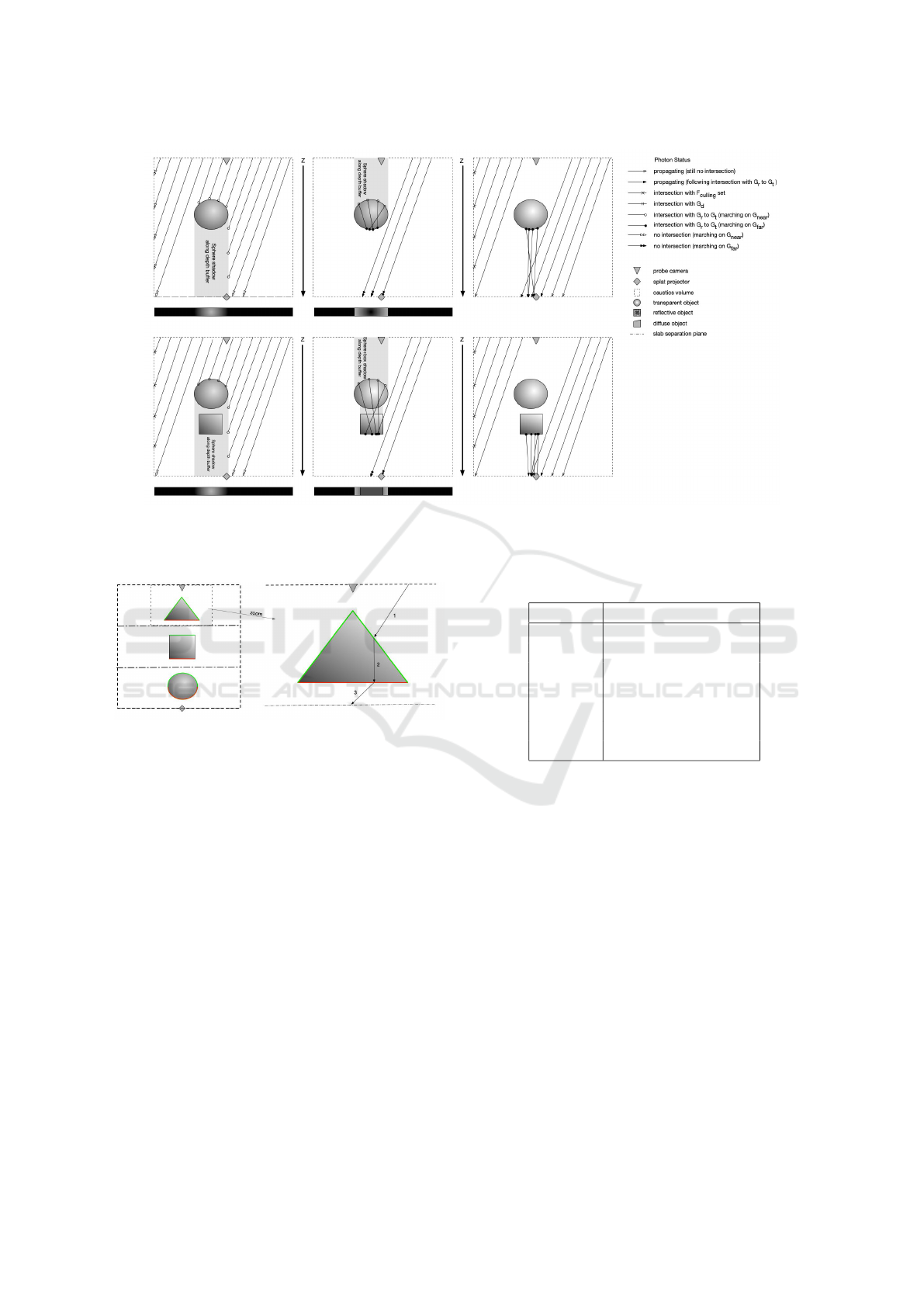
Figure 1: Top row shows three stages of propagating photons over G
near
(1
st
column), G
f ar
(2
nd
column), and resulting
photon paths (3
rd
column). The second row show the same scene with a refractive box added under the sphere. Note how the
G
f ar
buffer changes to account for the box and how the resulting photon paths are similar to those in the previous row.
Figure 2: Right: Three slab configuration for an arbitrary
bounding volume, the green and red lines highlight what
geometry is stored in G
near
and G
f ar
respectively. Left: ray
marching procedure within a single slab.
space; a depth test is carried out against G
near
to de-
tect intersections along the trajectory of the photon. If
the test fails, traversal continues until the photon in-
tersects the boundary of the slab. If a photon arrives
at the boundary that subdivides the caustics volume,
it is carried forward to the adjacent slab. If the bound-
ary intersected by the photon is also the boundary of
the caustics volume, then, depending on the assigned
attribute, the photon may be either terminated (colli-
sion with a culling face) or scheduled for rendering
(collision with an exit face).
Now we will consider what happens when the in-
tersection test with the G
near
depth buffer succeeds
and the surface is transmissive: although the photon
may be at a media interface, the test is not conclusive.
The photon might be passing behind the object with-
out going through it. To make the test more robust,
Table 2: Photon attributes.
Attribute Description
P
rad
Energy
P
pos
Position
P
dir
Direction
P
nrm
Surface normal
P
len
Current path length
P
grid
Density grid tile index
P
med
Photon medium
a further depth test is carried out against G
f ar
; if the
photon position is between the depth values sourced
from G
near
and G
f ar
, then we assume it is at a media
interface. The next thing to ascertain is whether the
photon is going from air to dielectric medium or vice-
versa. The photon attribute P
med
(see Table 2) is used
to tell whether a photon is inside a dielectric medium
or outside. Thus, if P
med
is false, and the surface nor-
mal at the interface lies in the opposite hemisphere
as the photon direction, we assume the photon is at
an air-dielectric medium interface and is entering the
denser medium. Conversely, if P
med
is true, the pho-
ton is inside the denser medium (inside a transmissive
object); if the surface normal at the interface lies in
the same hemisphere as the photon direction, then we
assume the photon is exiting the denser medium.
In both cases, if the surface normal tests fail, the
interface is ignored and the photon is assumed to re-
main in the original medium, air when P
med
is false
A Lightweight Photon Tracing Method for Visualising Caustics
191

and the dielectric when P
med
is true.If an intersection
is recorded, the photon trajectory is amended to ac-
count for a change in medium or a reflection, when
the surface material is either transmissive or specu-
larly reflective. When a diffuse surface is encountered
at an intersection, the photon path is terminated; the
photon is then scheduled for rendering if it had been
earlier tagged as contributive. To account for trans-
missive objects that are entirely contained within a
single slab, ray marching switches to testing exclu-
sively against G
f ar
after the first recorded intersec-
tion. When all photons have been marched through
the slab, those with recorded intersections are propa-
gated to the boundaries of the slab.
3.4 Photon Splatting
The photon tracing process moves to the last step
when all input photons have reached either an exit or
a culling face. The former are scheduled for render-
ing via projectors, which are assigned to each of the
faces in F
exit
; any photon that exits the volume at one
of these faces is associated with the respective pro-
jector. In a sense, we emulate the generation process
of a cube-map, in a similar fashion to that applied by
(Ganestam and Doggett, 2015). For each projector,
a g-buffer is generated, capturing the scene from the
respective side of the caustics volume. Each photon
in the projector is marched to find the closest point of
intersection in the g-buffer; the position and surface
normal at the point of intersection are recorded and
used for photon density estimation and later, splatting.
For density estimation, the g-buffer is split into a grid
of square tiles. This is naive at best, and interested
readers are directed to more accurate techniques pro-
vided in (Mara et al., 2013). Each contributive photon
that has intersected the scene geometry, will be repre-
sented as splats. Splats are represented by quads with
a circular texture. However, the quad is not uniform
but adjusted according to the ray length and density
estimate. Orthogonal basis for each quad are con-
structed, namely from the surface normal at the inter-
section, the projection of the intersection direction at
the plane defined by the surface normal and the third
vector is the cross products of the previous two vec-
tors as detailed in (Haines and Akenine-Moller, 2019)
and (Adam Marrs and Wald, 2021). Finally, once all
photons have been rendered as oriented quads in a dif-
ferent frame-buffer, a Gaussian kernel is applied to
smoothen the result.
Photons are distributed evenly over the F
entry
sur-
face of the caustics volume and seeded with the cur-
rent direction of the light that is associated with the
volume. If there is more than one light, the pho-
ton pool is divided equally between all the contribut-
ing lights. Other sampling techniques can be utilised
(Shirley and Morley, 2003).
3.5 Optimisations
Algorithmic optimisations have been introduced to
improve the performance of the technique. Volumes
that are close to the camera are prioritised, by keeping
the slab count to the explicit number specified by the
user. However, if the volume is further away from the
camera, we make use of level-of-detail to reduce the
amount of slabs for the given volume. In case the vol-
ume is out of the camera frustum, we do not render
the photons for the respective volume.
Differential updates were introduced to the caus-
tics volume; as the volume is split into distinct slabs,
we only need to update any of the slabs in which a
change has occurred. As such, if we have 5 slabs
and a change occurred in the 5
th
slab, we would only
require to update slab 5 and the projectors. If light-
related updates occur in the scene, this optimisation
is not applicable and the whole propagation cycle is
executed.
4 RESULTS
Results address runtime performance and scalabil-
ity for different execution parameters. Specifically,
we show how the method scales for different pho-
ton counts, polygon counts and geometry buffer sizes.
Furthermore, we compare, qualitatively, results ren-
dered using our method in the Unity game engine to
renders using Blender. The system has been tested on
fives different scenes, which consist of transmissive or
reflective objects inside a Cornell Box variants; these
have been labelled as diamond (2K polygons), ring
(2.9K polygons), glass-ball (4K polygons), Suzanne
(97K polygons) and floating blocks (47.6K polygons).
Experiment Setup. For all performance tests, the fol-
lowing g-buffer resolutions (G
dims
) were used: 100 ×
100, 200 × 200 and 500 × 500 pixels. The higher
G
dims
, the more accurate the output is expected to be.
The tests were run using the following input photon
counts (
|
P
i
|
): 10K, 20K and 50K. A higher number
of input photons is expected to generate more defined
caustics formations and patterns at the cost of runtime
performance. The number of partitions of the caus-
tics volume (N
slabs
) was varied between 1 and 3 slabs.
The number of slabs is expected to guide the level
of refinement of the algorithm; a higher number of
GRAPP 2022 - 17th International Conference on Computer Graphics Theory and Applications
192
slabs means that the interactions of photons and com-
plex geometry may be better captured and modelled,
whereas a lower number of slabs yields a coarser rep-
resentation of the actual interactions. A steep cost is
associated with an increased number of slabs as each
traversal requires expensive state copies from GPU to
CPU, for photons to be filtered and passed on to the
next slab or projector(s).
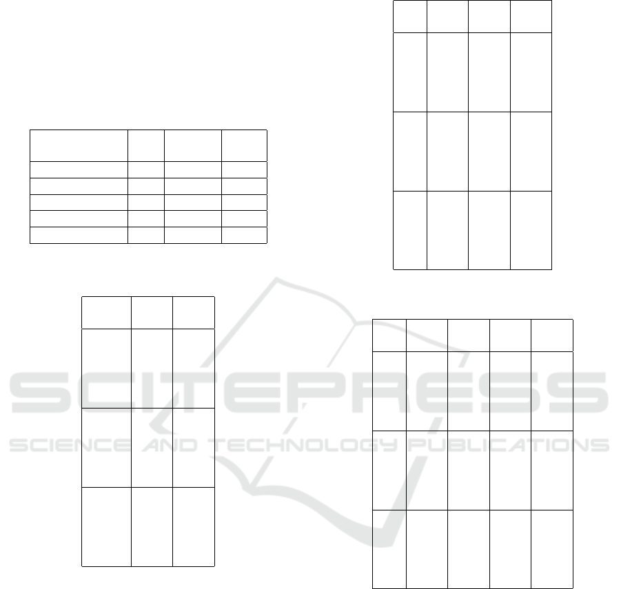
Table 3: Timings for the offline renders.
Scene Ref Sample Time
Count mins
diamond A 2000 5:41
ring B 2000 9:56
glass-ball C 2000 5:20
Suzanne D 2000 6:41
floating Blocks E 2000 6:21
Table 4: Timing and performance results for one-slab caus-
tics volume.
Scene S
1
Proj
(ms) (ms)
A 48 47
B 54 44
C 22 18
D 72 62
E 54 50
A 53 52
B 64 45
C 56 52
D 93 69
E 58 54
A 53 52
B 64 45
C 56 52
D 93 69
E 58 54
Performance. Tables 4, 5 and 6 show the perfor-
mance results for the five scenes, and highlight the
cost of projection passes for the respective photon
paths. Costs are expressed in ms. Each table con-
tains three different sets of results that vary according
to G
dims
(g-buffer size) and P
i
(photon count) and the
following combinations were used: 100
2
and 10K,
200
2
and 20K and finally 500
2
and 50K. Optimisa-
tions (see 3.5) were disabled for these tests. A full up-
date of the caustics volume was enforced on each and
every change in the lighting or scene geometry. As
expected, an increase in quality settings (higher G
dims
,
N
slabs
and
|
P
i
|
) result in a decrease in runtime perfor-
mance, directly impacting the average frame rate of
the main rendering pipeline. For simple scene config-
Table 5: Timing and performance results for two-slab caus-
tics volume.
Sc. S
1
S
2
Proj
(ms) (ms) (ms)
A 44 46 43
B 49 49 52
C 47 52 72
D 82 63 72
E 77 56 67
A 53 50 48
B 52 67 40
C 60 50 50
D 92 78 71
E 84 72 68
A 56 62 58
B 61 104 47
C 62 59 70
D 141 113 117
E 130 100 105
Table 6: Timing and performance results for three-slab
caustics volume.
Sc. S
1
S
2
S
3
Proj
(ms) (ms) (ms) (ms)
A 48 46 46 49
B 37 41 42 43
C 20 17 20 14
D 64 53 46 58
E 65 56 57 65
A 52 60 51 44
B 49 72 49 50
C 49 71 49 47
D 78 69 66 60
E 81 69 68 71
A 75 62 63 63
B 58 107 58 54
C 92 76 74 73
D 124 103 92 95
E 141 106 104 102
urations (ring, glass ball and diamond) with low poly-
gon counts, a single slab was enough to visualise the
caustics pattern. Increasing the slab count for these
scenes did not increase the quality of the pattern, but
was rather detrimental in that performance was im-
pacted at the cost of no visible benefit.
Image Comparison. The quality of rendered caus-
tics was compared to reference images of the same
scenes generated using Blender (see Figure 3). These
images were path-traced; specifically, LuxCore was
used to ensure high quality caustics in the output. The
best quality settings were used to generate images us-
ing out method: g-buffer resolution was set to 500
A Lightweight Photon Tracing Method for Visualising Caustics
193
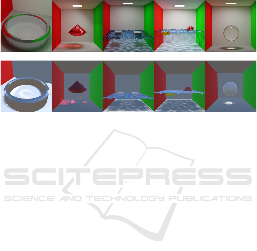
Figure 3: Top row: Test scenes rendered using Blender and LuxCore. Bottom row: Test scenes rendered using our implemen-
tation in Unity3D.
× 500, the photon count to 50K and the caustics vol-
ume partitioned into three slabs. The offline rendering
times for the reference images are shown in Table 3.
There are noticeable differences between the caustics
in the reference images and those generated using our
method; nevertheless, images generated by the latter
were rendered in a fraction of the time taken to render
the references. In our method, a naive photon splat-
ting algorithm was used with a simple density estima-
tion (3.4); replacing this with state of the art methods
could yield a better caustics visualisation.
Discussion. Fast interactive rendering of dynamic
caustics is still a holy grail in real time rendering.
Hardware accelerated ray tracing has pushed the en-
velope further and brought us closer to a solution;
nevertheless, this excludes a plethora of devices, par-
ticularly portable devices and platforms without the
latest GPU hardware advancements. The presented
method does not require any ray tracing hardware; in-
stead, it employs screen-space ray marching to com-
pute photon traversal through the volume. The par-
titioning of the caustics volume into slabs serves a
twofold goal: the amortisation of computation over a
number of frames and geometry refinement. Further-
more, only slabs affected by dynamic scene changes
are considered during updates. A progressive ap-
proach was also presented, where a fraction of the
total number of photons is traversed per update, up
to some maximum count, to preserve frame rates in
weak and low-end devices. The image comparison
shows that although some caustics formations are cor-
rectly captured by our method, it is still an approxi-
mation that has correctness and numerical limitations.
Caustics visualised on the sides walls of the Cornell
box in LuxCore rendered scenes could not be visu-
alised with the caustics volume due to the light sam-
pling method utilised.
5 CONCLUSION
In this paper we have proposed a lightweight method
for photon tracing aimed at visualising caustics. The
results show that the method is promising notwith-
standing the clear room for optimisation in our im-
plementation.
The approximative nature of the method is such
that certain paths cannot be modelled; for instance,
back reflections, or light paths that are reflected back
in the general direction of the light source, cannot
be accurately modelled. To do so, further render-
ing passes would be required, potentially impacting
performance. This limitation also affects a transpar-
ent medium that is embedded within another trans-
parent medium; for each slab, it is assumed that at
most two media interfaces exist. Updates to slabs in
the caustics volume are ordered. Therefore, in a full
update, n slabs require n + 1 iterations; when the it-
erations are amortised over a number of frames, the
resulting caustics appear to be trailing behind updates
to light sources or geometry that triggered the up-
date. Optical Flow (Horn and Schunck, 1981) could
be employed to predict the general direction of mo-
tion and extrapolate the pattern, thus reducing the ap-
parent lag. Furthermore, pipelined parallelism could
be introduced, to compute slabs from different itera-
tions concurrently, similar to how instructions are ex-
GRAPP 2022 - 17th International Conference on Computer Graphics Theory and Applications
194

ecuted in a RISC CPU pipeline. This would also re-
quire substantial improvement to the current photon
tracing implementation. Plausibility does not entail
correctness: implementing photon tracing using ray
tracing, hardware accelerated also, would enable us
to measure the accuracy of the solution and quantify
the fidelity of the resulting caustics formations.An in-
teresting avenue to explore is the light transport be-
tween different caustics volumes in the scene; at the
moment, these volumes are independent of one an-
other. Furthermore, integration into distributed ren-
dering pipelines is another avenue worth exploring,
especially in the context of VR rendering systems,
which would greatly benefit from the added realism
provided by caustics.Finally, the current implemen-
tation would greatly benefit from optimisation, to fur-
ther minimise frame rates and make it suitable for ren-
dering on low-end devices.
ACKNOWLEDGMENTS
This work was supported by the Notarial Archives of
Malta.
REFERENCES
Adam Marrs, P. S. and Wald, I. (2021). Ray tracing gems 2.
chapter 30. Apress.
Arvo, J. et al. (1986). Backward ray tracing. In Develop-
ments in Ray Tracing, Computer Graphics, Proc. of
ACM SIGGRAPH 86 Course Notes, pages 259–263.
Bugeja, K., Debattista, K., and Spina, S. (2019). An asyn-
chronous method for cloud-based rendering. The Vi-
sual Computer, 35.
Crassin, C., Luebke, D., Mara, M., McGuire, M., Oster,
B., Shirley, P., Sloan, P.-P., and Wyman, C. (2015).
CloudLight: A system for amortizing indirect lighting
in real-time rendering. Journal of Computer Graphics
Techniques (JCGT), 4(4):1–27.
Dachsbacher, C. and Stamminger, M. (2006). Splatting in-
direct illumination. In Proceedings of the 2006 Sym-
posium on Interactive 3D Graphics and Games, I3D
’06, page 93–100, New York, NY, USA. Association
for Computing Machinery.
Doghramachi, H. (2020). Lighting technology of the last
of us part ii. In ACM SIGGRAPH 2020 Talks, SIG-
GRAPH ’20, New York, NY, USA. Association for
Computing Machinery.
Evangelou, I., Papaioannou, G., Vardis, K., and Vasilakis,
A. A. (2020). Rasterisation-based progressive photon
mapping. In The Visual computer (2020).
Ganestam, P. and Doggett, M. (2015). Real-time multiply
recursive reflections and refractions using hybrid ren-
dering. 31(10):1395–1403.
Haines, E. and Akenine-Moller, T. (2019). Ray tracing
gems: High-quality and real-time rendering with dxr
and other apis. chapter 24. Apress.
Horn, B. and Schunck, B. (1981). Determining optical flow.
Artificial Intelligence, 17:185–203.
Ihrke, I., Ziegler, G., Tevs, A., Theobalt, C., Magnor, M.,
and Seidel, H.-P. (2007). Eikonal rendering: Efficient
light transport in refractive objects. SIGGRAPH ’07:
ACM SIGGRAPH 2007 papers, page 59.
Jarosz, W., Nowrouzezahrai, D., Thomas, R., Sloan, P.-P.,
and Zwicker, M. (2011). Progressive photon beams.
ACM Trans. Graph., 30(6):1–12.
Jensen, H. W. (1996). Global illumination using photon
maps. In Pueyo, X. and Schr
¨
oder, P., editors, Ren-
dering Techniques ’96, pages 21–30, Vienna. Springer
Vienna.
Kajiya, J. T. (1986). The rendering equation. SIGGRAPH
Comput. Graph., 20(4):143–150.
Lafortune, E. and Willems, Y. (1998). Bi-directional path
tracing. Proceedings of Third International Confer-
ence on Computational Graphics and Visualization
Techniques (Compugraphics’, 93.
Liktor, G. and Dachsbacher, C. (2011). Real-time volume
caustics with adaptive beam tracing. In Symposium on
Interactive 3D Graphics and Games, I3D ’11, page
47–54, New York, NY, USA. Association for Com-
puting Machinery.
Magro, M., Bugeja, K., Spina, S., and Debattista, K. (2020).
Cloud-based dynamic gi for shared vr experiences.
IEEE Computer Graphics and Applications, PP:1–1.
Mara, M., Luebke, D., and McGuire, M. (2013). To-
ward practical real-time photon mapping: Efficient
gpu density estimation. In Proceedings of the ACM
SIGGRAPH Symposium on Interactive 3D Graphics
and Games, I3D ’13, page 71–78, New York, NY,
USA. Association for Computing Machinery.
Shirley, P. and Morley, R. K. (2003). Realistic Ray Tracing.
A. K. Peters, Ltd., USA, 2 edition.
Sriwasansak, J., Gruson, A., and Hachisuka, T. (2018). Effi-
cient energy-compensated vpls using photon splatting.
Proc. ACM Comput. Graph. Interact. Tech., 1(1).
Umenhoffer, T. (2008). Caustic triangles on the gpu.
A Lightweight Photon Tracing Method for Visualising Caustics
195
