Preserving Order during Crossing Minimization in Sugiyama Layouts
S
¨
oren Domr
¨
os
a
and Reinhard Von Hanxleden
b
Department of Computer Science, Kiel University, Kiel, Germany
Keywords:
Sugiyama Layout, Layered Drawings, User Intentions, Graph Order.
Abstract:
The Sugiyama algorithm, also known as the layered algorithm or hierarchical algorithm, is an established
algorithm to produce crossing-minimal drawings of graphs. It does not, however, consider an initial order of
the vertices and edges. We show how ordering real vertices, dummy vertices, and edge ports before crossing
minimization may preserve the initial order given by the graph without compromising, on average, the quality
of the drawing regarding edge crossings. Even for solutions in which the initial graph order produces more
crossings than necessary or the vertex and edge order is conflicting, the proposed approach can produce better
crossing-minimal drawings than the traditional approach.
1 INTRODUCTION
Edge crossings are the most important syntactic aes-
thetic criterion for node-link diagrams (Purchase,
1997). However, the desire for few edge crossings
should not hinder us in synthesizing, automatically
and in real-time, a diagram that abides the Nothing
is Obviously Non-Optimal (NONO) principle (Kief-
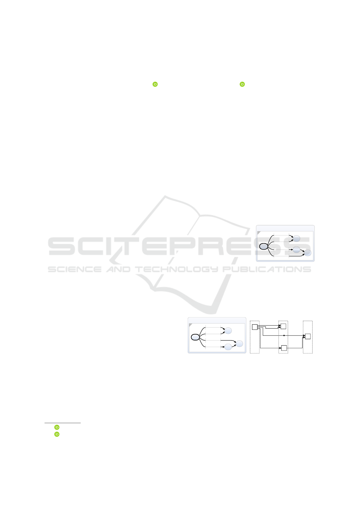
fer et al., 2016). The SCChart (von Hanxleden et al.,
2014) in Figure 1b has no edge crossings, but the
drawing is obviously non-optimal when considering
the transition order specified in the textual source in
Figure 1a. Specifically, the order of edges in the draw-
ing is not consistent with the order of the correspond-
ing transitions in the graph.
In general, graph drawing algorithms consider
graphs to consist of unordered sets of vertices and
edges. This is also the case for the Sugiyama algo-
rithm (Sugiyama et al., 1981), also known as the lay-
ered or hierarchical algorithm, that is used to produce
the drawing in Figure 1b. However, in practice we
often want to consider some ordering, e. g. the tex-
tual order defined in some input file, e. g. in a textual
SCChart depicted in Figure 1a. This paper presents
an approach to produce drawings where the edges
and vertices are ordered in the graph model whenever
that is possible without increasing the number of edge
crossings, see Figure 1c.
Preserving the textual order in the diagram is part
of secondary notation (Petre, 1995) since the visual
a
https://orcid.org/0000-0002-8011-8484
b
https://orcid.org/0000-0001-5691-1215
1 scchart Example1 {
2 output int O
3 initial state init // v
1
4 do O = 1 go to s1 // e
11
5 do O = 2 go to s1 // e
12
6 do O = 3 go to s3 // e
13
7 do O = 4 go to s2 // e
14
8
9 state s1 // v
2
10
11 state s2 // v
3
12 go to s3 // e
31
13
14 state s3 // v
4
15 }
(a) Textual SCChart input file
Example1
init
s1
s2
s3
1: / O = 1
2: / O = 2
4: / O = 4
3: / O = 3
-
(b) SCChart synthesized
from textual input with
Sugiyama layout not con-
sidering order
Example1
init
s1
s2
s3
1: / O = 1
2: / O = 2
4: / O = 4
3: / O = 3
-
(c) SCChart considering
order (this work)
v1
v2
v3
v4
e11
e12
e14
e13
e31
Layer 1 Layer 2 Layer 3
d1
(d) The underlying graph
Figure 1: An SCChart with an underlying ordered
graph G = (V, E) with V = hv
1
, v
2
, v
3
, v
4
i and E =
hhe
11
, e
12
, e
13
, e
14
i, hi, he
31
i, hii.
complies with the semantics. Furthermore, since ver-
tices and edges are ordered as in the graph model, we
expect that the layout stability, and with it the preser-
vation of the mental map (Eades et al., 1991; Misue
et al., 1995), is improved, since small changes in the
156
Domrös, S. and Von Hanxleden, R.
Preserving Order during Crossing Minimization in Sugiyama Layouts.
DOI: 10.5220/0010833800003124
In Proceedings of the 17th International Joint Conference on Computer Vision, Imaging and Computer Graphics Theory and Applications (VISIGRAPP 2022) - Volume 3: IVAPP, pages
156-163
ISBN: 978-989-758-555-5; ISSN: 2184-4321
Copyright
c
 2022 by SCITEPRESS – Science and Technology Publications, Lda. All rights reserved

graph model do not cause large changes in the draw-
ing.
1.1 Contribution & Outline
This paper presents an approach to introduce the
concept of graph order to the Sugiyama algorithm.
Specifically, the contributions are the following:
• we define the concept of vertex and edge graph
order (Section 3.1);
• we adapt crossing minimization for proper lay-
ered ordered graphs (Section 3.2);
• we extend the proposed solution to include par-
tially ordered graphs (Section 3.3);
• we extend the solution to include backward edges
(Section 3.4);
• we propose an order metric that can be used to fur-
ther improve crossing minimization (Section 3.5).
The resulting algorithm configurations are discussed
and evaluated in Section 4. Section 5 presents related
work and Section 6 concludes this paper.
An extended version of this paper has appeared
as a technical report (Domr
¨
os and von Hanxleden,
2021). Specifically, that report presents how to deal
with dangling source vertices and discusses various
insights in more detail.
2 LAYERED ALGORITHM
We define a graph G = (V, E), vertices V =
{v
1
, . . . , v
n
}, edges E ⊆ P × P, and ports P that the
edges are anchored at, where P(v) is the subset of
ports that belong to a vertex v. Conversely, v(p) ∈ V
denotes the vertex that port p is anchored at. For
an edge e = (p, q), p
s
(e) = p ∈ P(v) describes the
source port and p
t
(e) = q ∈ P(w) describes the tar-
get port. For simplicity, we also write e = (v, w) for
source vertex v and target vertex w as short form of
e = (p, q), v(p) = v, and v(q) = w if we do not care
about the ports. For port p, type(p) ∈ {src, tgt} indi-
cates whether p is a source or target port and e(p) ∈ E
returns the edge of the port p.
The algorithm places vertices in vertical layers, as
seen in Figure 1d, and only routes edges between two
layers, i. e. in-layer edges are forbidden. The algo-
rithm is divided into five phases: cycle breaking, layer
assignment, crossing minimization, vertex placement,
and edge routing (Sugiyama et al., 1981). The first
two phases transform the digraph into a proper lay-
ered digraph. In a layered graph G = (V, E, L) the
set of vertices V is partitioned into m mutually ex-
clusive ordered subsets that represent their layering
L = (L
1
, . . . , L
m
), with L
i
= hv
L
i1
, . . . , v
L
ir
i for a layer
of size r. L(v) = i denotes the layer i of a vertex
v ∈ V . A graph is proper layered iff for all edges
e = (v, w) ∈ E, L(w) = L(v) + 1 holds. Since this is
generally not possible for digraphs, dummy vertices
and dummy edges are added to replace long edges that
span multiple layers. In Figure 1d, the edge from v
1
to v
4
is a long edge with one dummy vertex d
1
in layer
2. We distinguish between real vertices and dummy
vertices.
We call vertices with no incoming edges sources
and vertices with no outgoing edges sinks, and define
the functions indegree : V → N and outdegree : V →
N that return the number of incoming and outgoing
edges of a vertex.
Cycle breaking transforms a given graph into an
acyclic one. This problem is commonly known as the
minimum feedback arc set problem and is NP-hard
(Karp, 1972). We call the edges that are reversed in
this process backward edges. In the following algo-
rithm, they are handled as normal edges. During the
edge routing phase, they are reversed to their original
direction.
The layer assignment phase creates a proper
layered graph by introducing dummy vertices and
dummy edges.
Crossing minimization uses the proper layered di-
graph and orders all vertices in their layers and ports
on their vertices such that minimal edge crossings are
created, as seen simplified in Algorithm 1.
Algorithm 1: crossingMinimization (original).
Input: A proper layered graph G = (V, E, L)
Output: A proper layered ordered graph
1 r = randomSeed // A fixed random seed
2 t = 7 // Thoroughness
3 sweepForward = sweepDirection(r)
4 bestOrder = null
5 for i = 0; i < t;i = i + 1 do
6 G = randomizeLayers(G, r,sweepForward)
7 do
8 foreach L
i
∈ L do
9 minimizeCrossings(L
i
)
10 while improved(G);
11 if crossings(G) < crossings(bestOrder) then
12 bestOrder = G
13 sweepForward = ¬sweepForward
14 return bestOrder
Since the crossing minimization problem is NP-
hard and remains NP-hard on bipartite graphs (Garey
and Johnson, 1983), a heuristic that includes ports
(Sp
¨
onemann et al., 2010) is used. Crossing minimiza-
Preserving Order during Crossing Minimization in Sugiyama Layouts
157

tion consists of several runs to prevent local minima
bounded by the thoroughness value t. Seeded random
values are used to guarantee the same diagram for the
same graph. For the first run it is randomly decided
whether the layers are traversed beginning with the
first or the last layer. We call this the sweep direc-
tion and distinguish between a forward sweep and a
backward sweep. Moreover, the random seed is used
to reorder all independent vertices and ports, i. e. all
sources or sinks and their ports, via randomizeLayers.
In this algorithm, edges are ordered via the ports they
are anchored at. Since edges only connect ports in
neighboring layers, ordering the ports is enough and
edge order is defined by them.
Random permutation of the first or last layer is
applied to prevent local minima. If the random initial
order yields a local minimum it can be resolved by
using a higher thoroughness value or by permuting
the first layer. The thoroughness value of 7 proved to
be sufficient to prevent local minima even for large
graphs in its implementation in the Eclipse Layout
Kernel (ELK)
1
.
We call the current layer the fixed layer and the
next layer (in case of a forward sweep L
i+1
, else L
i−1
)
the free layer. At this point we consider the layers or-
dered and use a crossing minimization strategy, such
as the barycenter heuristic (Sp
¨
onemann et al., 2010),
to order the vertices and ports in the free layer and
continue to do so with the next layer while sweeping
forward and backward until no improvement can be
found. For each run the resulting edge crossings are
counted efficiently by using the order of their ports, as
described by (Barth et al., 2004). The run that yields
the smallest number of crossings defines the order of
the vertices in each layer and the order of the ports on
each vertex.
To evaluate our approach we use the Barycen-
ter method proposed by Sugiyama et al. to minimize
the crossings. However, any approach that does not
change the vertex order if it is crossing minimal would
work here, such as the median heuristic (Eades and
Wormald, 1986) or any approach that sweeps through
the layers and counts crossings to compare the result.
3 GRAPH ORDER CROSSING
MINIMIZATION
As explained earlier, a key difference between the
standard layered approach and our proposal is that
we consider vertices and edges to be ordered. The
next section will formalize this order. This serves
1
https://www.eclipse.org/elk/
as grounding for the subsequent sections, which ex-
plain how to produce drawings that aim to reflect that
order whenever this is possible without compromis-
ing other aesthetic criteria, specifically the number of
edge crossings.
3.1 Graph Order
Definition 1 (Ordered Graph). We de-
fine an ordered graph as G = (V, E) were
V = hv
1
, . . . , v
n
i is the ordered set of vertices
and E = hhe
11
, . . . , e
1k
1
i, . .. , he
n1
, . . . , e
nk
n
ii is the
ordered set of ordered sets of k
i
outgoing edges for
each vertex v
i
. E implicitly defines an ordered set of
outgoing and incoming ports P at which each edge is
anchored.
An example of an ordered graph that follows Def-
inition 1 can be seen in Figure 1. A proper layered
ordered graph G = (V, E, L) is defined analogously.
We define o : V ∪ E ∪ P → Z (see Definition 2) as the
function that assigns a graph order value to vertices,
edges, and ports.
Definition 2 (Graph Order o). o(v) = n if v ∈ V is
the nth vertex in the graph. Analogously, o(e) = n if
e ∈ E is the nth edge in the graph and o(p) = o(e(p))
for port p ∈ P.
The graph order specifies orders for vertices and
edges, as expressed by o. Ideally, this graph order
is also reflected in the drawing of the graph, as is
the aim of this work. However, this is not always
possible, at least not simultaneously for both vertices
and edges, as they may sometimes induce conflict-
ing orderings, as illustrated in the example in Fig-
ure 2. Actually one might argue that such cases
could and should be avoided, e. g. when writing a
textual SCCharts specification, but we still want to
be able to handle such cases. We, therefore, distin-
guish the graph order on vertices and edges from the
drawing order defined by a vertex order ≺
v
: V × V
and a port order ≺
p
: P × P. We also introduce a
flag prioEdgeOrder = ¬prioVertexOrder to express
whether vertex or edge order is prioritized.
Definition 3 (Vertex Order ≺
v
for ordered graphs).
For v, w ∈ L
i
for some layer L
i
∈ L, we define ≺
v
such
that v ≺
v
w holds iff one of the following cases ap-
plies:
1. prioVertexOrder ∧ o(v) < o(w).
I. e. vertices are ordered by their graph order.
For example in Figure 1, we have v
2
≺
v
v
3
2. prioEdgeOrder ∧ p
s
(getFirstEdge(v)) ≺
p
p
s
(getFirstEdge(w)) where getFirstEdge re-
turns the edge on the first port of the vertex. The
IVAPP 2022 - 13th International Conference on Information Visualization Theory and Applications
158

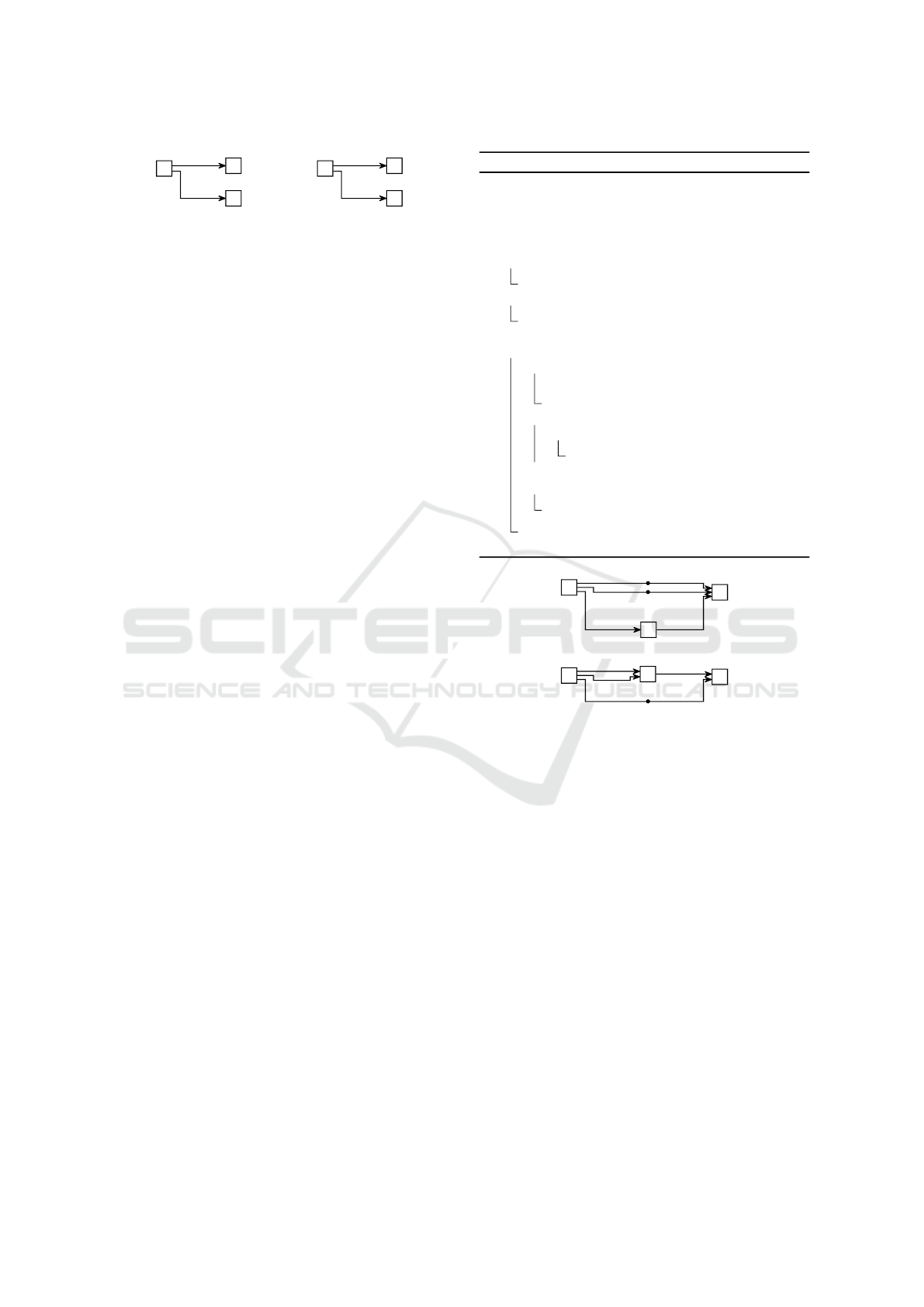
init
v1
v2
e12
e11
(a) Prioritize edge or-
der over vertex order
(prioEdgeOrder)
init
v1
v2
e12
e11
(b) Prioritize vertex
order over edge order
(prioVertexOrder)
Figure 2: We can either prioritize edge or vertex order. This
may yield different drawings depending on the graph order.
first edge is on the incoming port that was deemed
smallest by ≺
p
.
I. e. vertices are ordered by their incoming edges
and not by the graph order.
Definition 4 (Port Order ≺
p
). For ports a and b at-
tached to the same vertex v, v(a) = v = v(b), we define
≺
p
such that a ≺
p
b holds iff one the following cases
applies:
1. type(a) = type(b) = src ∧ v(p
t
(e(a))) =
v(p
t
(e(b))) ∧ o(a) < o(b).
I. e. means outgoing ports that connect to the
same target vertex are ordered by the graph order
of their edges.
2. type(a) = type(b) = src ∧ v(p
t
(e(a))) = w 6=
u = v(p
t
(e(b))) ∧ o(getMinEdge(v, w)) <
o(getMinEdge(v, u)) where getMinEdge :
V × V → E returns the edge with the minimum
graph order o between two vertices.
I. e. outgoing edges that do not connect to the
same target vertex are ordered by the minimal
edge order of their target.
E. g. this reduces unnecessary edge crossings
in Figure 3 since placing e
43
below e
42
would al-
ways produce a crossing and bundles edges with
the same target.
3. type(a) = type(b) = tgt ∧ p
s
(e(a)) ≺
p
p
s
(e(b)).
I. e. incoming ports are sorted as the corre-
sponding source port of their edge. This is needed
to prevent unnecessary crossings since the source
ports are already correctly ordered by ≺
p
.
3.2 Proper Layered, Ordered Graphs
Our goal is to order all ports and vertices before cross-
ing minimization. We change crossingMinimization
in Algorithm 1 such that the bestOrder is initialized
with the input graph G, the first run starts with a
forward sweep, and the second run with a backward
sweep, as seen in Algorithm 2. For these first two
runs randomizeLayers is not executed since the graph
is already ordered.
Algorithm 2: crossingMinimization (new).
Input: A proper layered graph G = (V, E, L)
Output: A proper layered ordered graph
1 r = randomSeed // A fixed random seed
2 t = 7 // Thoroughness
3 sweepForward = true
4 foreach v ∈ V do
5 sort(P(v), ≺
p
)
6 foreach L
i
∈ L do
7 sort(L
i
, ≺
v
)
8 bestOrder = G
9 for i = 0; i < t;i = i + 1 do
10 if i > 1 then
11 G =
randomizeLayers(G, r, sweepForward)
12 do
13 foreach L
i
∈ L do
14 minimizeCrossings(L
i
)
15 while improved(G);
16 if crossings(G) < crossings(bestOrder) then
17 bestOrder = G
18 sweepForward = ¬sweepForward
19 return bestOrder
v1
v2
v3
v4
v5
v6
e12
e11
e21
e41
e42
e51
e43
e13
Figure 3: Two graphs with long edges and multiple edges to
the same target. Edges with the same target are grouped to-
gether to reduce potential edge crossings, (dummy vertices
marked as black circles).
3.3 Partially Ordered Graphs
When long edges are introduced, the graph definition
changes and dummy vertices and edges are added that
have no graph order. A properly layered, partially
ordered graph G is defined as the tuple (V
0
, E
0
, L
0
)
with V
0
= (V,V
D
) with V
D
= {d
1
, . . . , d
n
} as the set
of dummy vertices, E
0
= (E
L
, E
D
) with E
L
the or-
dered set of edges in which long edges (v, w) are
replaced by shortened long edges (v, d
i
) and E
D
=
{e
d
1
, . . . , e
d
n
} the set of dummy edges. As before, P
0
contains the ports of the corresponding edges of E
0
.
L
0
= (L
0
1
, . . . , L
0
n
) with L
0
i
= (L
i
, L
D
i
) consists of the
ordered part L
i
and the set of dummy vertices L
D
i
in
that layer. Dummy vertices and edges are originally
not part of the graph and have, therefore, no derived
graph order. We extend o such that o(e
d
i
) = o(e
k j
)
Preserving Order during Crossing Minimization in Sugiyama Layouts
159

for a dummy edge e
d
i
if e
k j
is the original long edge
the dummy edge was created for. Note that a dummy
vertex has no defined graph order value.
We have to change cases 1 and 2 of Definition 4
to also handle long edges. Instead of comparing the
target vertex, the long edge target vertex, which corre-
sponds to the real vertex the edge eventually connects
to, of each port is compared.
Definition 3 also has to be changed. The condi-
tion in case 1 changes to (prioEdgeOrder ∨ c ∈
V
D
∨ u ∈ V
D
) ∧ v(p
s
(getFirstEdge(v))) ≺
v
v(p
s
(getFirstEdge(w))). Dummy vertices are
compared to other vertices using the incoming edges.
3.4 Backward Edges
Backward edges are in most cases already handled
by the algorithm. For a consistent drawing style, we
want to place backward edges below normal ones and
change Definition 4 case 1 such that this is the case,
and change getMinEdge in case 2 such that the graph
order of backward edges is not considered here since
they originate from a different vertex.
3.5 A Graph Order Metric
The defined relations ≺
v
and ≺
p
serve as a metric
to decide how good a graph is ordered. This metric
can be used as a secondary criterion during crossing
minimization. To do this, line 16 in Algorithm 2 is
changed by adding the port or vertex order violations
multiplied by a weight w
v
and w
p
, so that the condi-
tion becomes:
w
p
· portOrderViolations(G)
+ w
v
· vertexOrderViolations(G) + crossings(G)
< w
p
· portOrderViolations(bestOrder)
+ w
v
· vertexOrderViolations(bestOrder)
+ crossings(bestOrder)
where portOrderViolations and vertexOrder-
Violations count the number of port and vertex
order violations for a partially ordered graph. These
weights express how many order violations are as
important as an edge crossing. E. g. w
v
= w
p
= 0.1
means that 10 vertex or port order violations are as
important as an edge crossing.
4 EVALUATION
We compare nine different algorithm configurations,
as seen in Table 1. Note that N
V
and N
E
produce the
Table 1: N (unordered), V (prioVertexOrder), E
(prioEdgeOrder). Overview and encoding of the evaluated
algorithmic alternatives. Columns differ in whether vertices
or edges are prioritized, rows differ in the weights assigned
to vertex/port order violations relative to edge crossings,
which carry a weight of 1.
w
p
w
v
N V E
0 0 N
V
, N
E
V E
> 0 0 V
w
p
,0
E
w
p
,0
0 > 0 V
0,w
v
V
0,w
v
> 0 > 0 V
w
p
,w
v
E
w
p
,w
v
same graph but are differently evaluated regarding
their violations of the graph order, as described in
Section 4.2.
We consider 54 SCCharts that were developed by
humans. SCCharts models may consist of concurrent
more than one concurrent region with states and edges
between them. Each region has its own graph. For
each model we, therefore, might solve several graph
drawing problems. The chosen models have two to 72
vertices per region and up to 310 vertices per model
with an average of 44 vertices per model (including
dummy vertices). There are from one to 16 vertices
per layer. The edge density to adjacent layers is two
to 73 with an average of 9. The average vertex degree
is between zero and seven.
For all graphs the ordering step is done in a
fraction of a millisecond and is significantly quicker
and less complex than crossing minimization in gen-
eral. The layout direction is set the RIGHT and
the dummy vertices are sorted above normal vertices
(dummyVerticesAb ove ). How a value for w
v
and w
p
is chosen is described in the following.
4.1 Weighted Ordering with w
v
and w
p
Table 2 illustrates the effects of varying w
v
and w
p
on edge crossings and on the number of fully ordered
drawings of the 54 graphs. Increasing the weight of
≺
v
and ≺
p
during crossing minimization tends to in-
crease the number of correctly ordered graphs at the
cost of edge crossings, but it cannot always find an
ordering with minimal order violations. The reasons
for this is that the barycenter heuristic (or any other
commonly used approach) used during crossing min-
imization does not focus on the order but on crossing
minimization. If no run yields the ordered solution, it
cannot be chosen, even though it would be chosen if
it occurred, based on the weights w
v
and w
p
.
4.2 Quantitative Evaluation
The number of drawing order violations for the dif-
ferent approaches can be seen in Table 2. N
V
serves
IVAPP 2022 - 13th International Conference on Information Visualization Theory and Applications
160

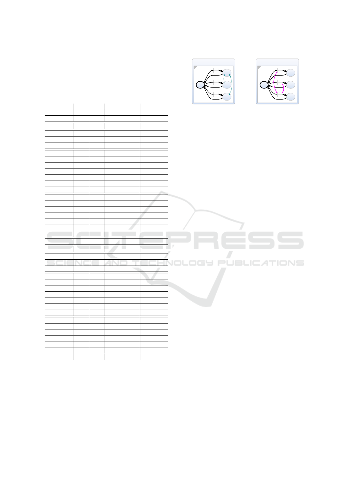
Table 2: Graph order violations for the metrics ≺
v
and ≺
p
for w
v
and w
p
set to 0.001, 0.01, 0.1, 0.5, 1, 10, and 100 for
their respective approaches. Lines for V
w
p
,0
and E
w
p
,0
are
omitted since they did not change with varying w
p
. Fully
ordered drawings describes the number of models that have
no order violations in any part of their model. Crossings
describes the total number of edge crossings in all regions
of all 54 models with the corresponding algorithm.
Fully ordered
≺
v
≺
p
drawings Crossings
N
V
250 695 1 26
V 143 91 23 32
V
0.001,0
143 91 23 32
. . . . . . . . . . . . . . .
V
100,0
143 91 23 32
V
0,0.001
91 173 24 28
V
0,0.01
91 173 24 28
V
0,0.1
91 173 24 28
V
0,0.5
44 172 24 28
V
0,1
81 184 25 39
V
0,10
64 159 26 82
V
0,100
72 169 26 112
V
0.001,0.001
122 96 24 28
V
0.01,0.01
122 96 24 28
V
0.1,0.1
122 96 24 28
V
0.5,0.5
95 78 26 36
V
1,1
102 48 29 93
V
10,10
129 12 29 149
V
100,100
129 12 29 149
N
E
45 695 1 26
E 27 91 31 32
E
0.001,0
27 91 31 32
. . . . . . . . . . . . . . .
E
100,0
27 91 31 32
E
0,0.001
14 93 32 28
E
0,0.01
14 93 32 28
E
0,0.1
14 93 32 28
E
0,0.5
10 88 32 28
E
0,1
10 101 33 32
E
0,10
12 101 33 36
E
0,100
10 95 33 34
E
0.001,0.001
14 92 32 28
E
0.01,0.01
14 92 32 28
E
0.1,0.1
14 92 32 28
E
0.5,0.5
12 78 33 34
E
1,1
13 52 39 46
E
10,10
32 20 39 92
E
100,100
32 20 39 92
as a baseline for all approaches that have
prioVertexOrder set (i. e. V and V
w
p
,w
v
), N
E
serves as
a baseline for approaches with prioEdgeOrder (i. e. E,
E
w
p
,w
v
). The resulting drawing of N
V
and N
E
is the
same, we only count the ≺
v
violations by comparing
the graph order of real vertices in the N
V
case and
use the edge graph order for N
E
. All approaches that
prioritize edge order have, therefore, fewer vertex
order violations.
Example2
v1 v2
v3
v4
2.
3.
1.
-
(a) A drawing with
two ≺
v
violations for
a prioVertexOrder ap-
proach and none with
prioEdgeOrder.
Example2
v1
v2
v3
v4
2.
3.
1.
-
(b) A drawing with two ≺
p
violations.
Figure 4: Vertex order violations are shown in teal and edge
order violations in magenta.
Figure 4 visualizes how ≺
v
and ≺
p
order viola-
tions are counted for the different approaches. In Fig-
ure 4a, the shown vertex order violations are only
counted for all prioVertexOrder approaches since
prioEdgeOrder approaches order vertices by their in-
coming edges. In Figure 4b, we see two edge order
violations. Furthermore, note that the V approach
would not produce this drawing but the V
0,0.001
ap-
proach would. The V would initially order the ports
and vertices without creating violations (e. g. edge 1
above edge 2 and 3). If crossing minimization starts,
the vertices v
2
to v
4
are in a free layer and their order
is changed to comply with the port order to not pro-
duce additional crossings. For the V
0,0.001
approach
this creates two violations. The second run would
then yield the drawing in Figure 4b since v
2
to v
4
are
in the fixed layer for a backward sweep. The resulting
drawing has no vertex order violations and no cross-
ings and is, therefore, better than Figure 4a under the
V
0,0.001
approach.
The two approaches V
w
p
,w
v
and E
w
p
,w
v
that use the
≺
v
and ≺
p
metrics as a secondary criterion to edge
crossings have the fewest total number of order viola-
tions for their respective approaches, as seen in Table
2.
4.3 Qualitative Evaluation
The V approach is evaluated compared to the normal
approach. The results can be seen in Figure 5. Of
these 54 models, 31 were consistent and 23 were con-
flicting. 20 of the consistent models improved the or-
der and not just placed backward edges below normal
ones. This can also be an improvement if it intro-
duces a consistent drawing style but we chose to dis-
tinguish it from a real drawing order improvement.
Three of the models that had conflicts did not change
in the conflicting regions. 20 of the models that had
conflicts nonetheless improved the overall layout. Of
Preserving Order during Crossing Minimization in Sugiyama Layouts
161

●
Consistent models
●
Conflicting models
●
Order improved
●
Backwards edges below
11
3
20
5
15
Figure 5: Changes of the 54 evaluated models.
these 20 models, 15 had order improvements, the rest
just placed backward edges below normal edges. All
three conflicting models that did not improve, were,
by coincidence, ordered as good as possible.
4.4 Influence of Randomization
Table 2 shows that the N (unordered) approach has
fewer total crossings (26) than all other (ordered) ap-
proaches, even though we argue that ordering ver-
tices and ports before crossing minimization should
not necessarily increase the number of crossings rela-
tive to the traditional approach. As it turns out, four of
the 54 models have a different number of edge cross-
ings than the N approach. One has one crossing less
(from one to zero crossings), two have one crossing
more (from zero to one crossing), and another one
has either one or three additional crossings depend-
ing on the approach (from 15 to 16 or 18 crossings) in
some regions of some models. The reason for this is
randomization.
Randomization still has an influence on the quality
of the solution for some kind of graphs. If a graph is
conflicting or the drawing order produces additional
crossings, randomizeLayers is still used to create the
drawing, as seen in Algorithm 2. Therefore, these
graphs can by coincidence produce more or fewer
edge crossings or order violations.
In the ordered approach the first two runs do not
randomize the order and use the graph order for a for-
ward and backward sweep. The order after these two
sweeps is not the same order the unordered approach
uses for their first run. Therefore, the vertex and port
order is already different to the N approach before
randomization takes place. Since any kind random-
ization can lead to different results, some of these runs
can randomly be a local minimum or no longer be a
local minimum, and result in more or fewer crossings
or order violations. Only increasing the thorough-
ness reduces the probability of additional crossings
but does not solve this anomaly.
4.5 Evaluation
If one favors the edge order, E or E
w
p
,w
v
are the rec-
ommended approaches. For SCCharts E
w
p
,w
v
is rec-
ommended to still get better results if E falls back to a
random starting permutation. If one expects the user
to change the vertex order in the model file to create
the desired layout, V
0,w
v
should be used since it can
be used to enforce vertex positions.
The proposed approach performs especially good
for graphs that a tree-like with a final vertex were ev-
erything connects to (which might have a feedback
loop) or several feedback loops to the root vertex or
another central vertex. Without edge graph order, the
different routes trough the tree are not ordered by their
priority (e. g. the edge with priority 1 is on top, the
edge with priority 2 is below, ...), as the secondary no-
tation suggests, but randomly, which highly irritates
the user and impedes understandability since “true”
and “false” cases might change sides.
5 RELATED WORK
There were already several works that aim to iden-
tify or produce a human-like layout and operate at the
so called NONO principle (Nothing is obviously non-
optimal) (Kieffer et al., 2016). Kieffer et al. use this
principle and human participants to identify aesthetic
criterions and goals for a human-like orthogonal lay-
out algorithm. Purchase et al. (Purchase et al., 2020)
take this further and try to identify layouts that are ob-
viously machine made. We tackle similar goals. Fig-
ure 1b looks obviously machine made and is a draw-
ing a human would not produce. In contrast to Kieffer
et al., we choose to still use the layered algorithm and
try to conform with the NONO principle by using the
graph order as additional layout information to solve
obvious problems instead of developing a whole new
algorithm.
The are several extensions to the Sugiyama algo-
rithm. We will discuss some of them that aim to in-
fluence the order of vertices and edges.
(Waddle, 2001) uses constraints to order vertices
and to force them on specific positions even if this
causes additional crossings. We try to preserve the
initial order but still try to minimize crossings if pos-
sible. We focus on layout creation. Waddle, how-
ever, focuses on layout adjustment and prioritizes or-
der constraints over crossings. Our ordering does
not constrain the solution, but rather creates a bet-
ter crossing-optimal solution. They use layout adjust-
ment to maintain the mental map, we assume that the
graph order in the model file is a representation of the
modelers mental map.
(Mennens et al., 2019) aim to produce stable
drawings by maintaining a global order of vertices.
This global order constrains vertex movement in the
same layer. Again, this order will not be changed if
IVAPP 2022 - 13th International Conference on Information Visualization Theory and Applications
162

additional crossings are produced. Moreover, they do
not consider the ordering of edges, since there is at
most one edge from one vertex to another vertex.
(B
¨
ohringer and Paulisch, 1990) introduce absolute
and relative constraints to fix the order of vertices.
This is a viable solution to maintain graph order but
this, again, does not prevent additional crossings. We
want to automatically produce drawings that maintain
the graph order without causing additional crossings.
Again, B
¨
oringer and Paulisch do not constrain edges
but only vertices, which solves only one of our prob-
lems since no dummy vertices can be constrained.
6 CONCLUSION
We presented a solution to preserve the graph order
by setting an initially best ordering for crossing min-
imization. This allows us to maintain the graph or-
der without causing additional crossings introduced
by local minima other than through coincidence or or-
der constraints for many models.
Including the proposed graph order metric in the
crossing minimization step additionally to the cross-
ings as a secondary criterion seems beneficial. There-
fore, prioEdgeOrder with weighted vertices and ports
(E
w
p
,w
v
) is one potential option for SCCharts. An-
other one is V since it allows to control the layout
without changing the semantic by changing the vertex
graph order. Therefore, we make this setting config-
urable for SCCharts and to evaluate this further.
Future work on this project should evaluate
whether SCCharts that are created in a tool that vi-
sualizes the diagram taking the graph order into ac-
count results in more consistent models or otherwise
changes the way modelers design.
REFERENCES
Barth, W., Mutzel, P., and J
¨
unger, M. (2004). Simple and
efficient bilayer cross counting. Journal of Graph Al-
gorithms and Applications, 8(2):179–194.
B
¨
ohringer, K.-F. and Paulisch, F. N. (1990). Using con-
straints to achieve stability in automatic graph layout
algorithms. In Proceedings of the SIGCHI Conference
on Human Factors in Computing Systems, pages 43–
51, New York. ACM.
Domr
¨
os, S. and von Hanxleden, R. (2021). Preserving
order during crossing minimization in sugiyama lay-
outs. Technical Report 2103, Christian-Albrechts-
Universit
¨
at zu Kiel, Department of Computer Science.
ISSN 2192-6247.
Eades, P., Lai, W., Misue, K., and Sugiyama, K. (1991).
Preserving the mental map of a diagram. In Proceed-
ings of the First International Conference on Compu-
tational Graphics and Visualization Techniques, pages
34–43.
Eades, P. and Wormald, N. C. (1986). The median heuristic
for drawing 2-layered networks. Technical Report 69,
University of Queensland, Department of Computer
Science.
Garey, M. R. and Johnson, D. S. (1983). Crossing num-
ber is NP-complete. SIAM Journal on Algebraic and
Discrete Methods, 4(3):312–316.
Karp, R. M. (1972). Reducibility among combinatorial
problems. In Miller, R. E. and Thatcher, J. W., editors,
Complexity of Computer Computations (Proceedings
of a Symposium on the Complexity of Computer Com-
putations, March, 1972, Yorktown Heights, NY), pages
85–103. Plenum Press, New York.
Kieffer, S., Dwyer, T., Marriott, K., and Wybrow, M.
(2016). HOLA: human-like orthogonal network lay-
out. IEEE Trans. Vis. Comput. Graph., 22(1):349–
358.
Mennens, R. J., Scheepens, R., and Westenberg, M. A.
(2019). A stable graph layout algorithm for processes.
In Computer Graphics Forum, volume 38, pages 725–
737. Wiley Online Library.
Misue, K., Eades, P., Lai, W., and Sugiyama, K. (1995).
Layout adjustment and the mental map. Journal of
Visual Languages & Computing, 6(2):183–210.
Petre, M. (1995). Why looking isn’t always seeing: Read-
ership skills and graphical programming. Communi-
cations of the ACM, 38(6):33–44.
Purchase, H. C. (1997). Which aesthetic has the greatest
effect on human understanding? In Proceedings of the
5th International Symposium on Graph Drawing (GD
’97), volume 1353 of LNCS, pages 248–261. Springer.
Purchase, H. C., Archambault, D., Kobourov, S.,
N
¨
ollenburg, M., Pupyrev, S., and Wu, H.-Y. (2020).
The turing test for graph drawing algorithms. In Inter-
national Symposium on Graph Drawing and Network
Visualization, pages 466–481. Springer.
Sp
¨
onemann, M., Fuhrmann, H., von Hanxleden, R., and
Mutzel, P. (2010). Port constraints in hierarchical
layout of data flow diagrams. In Proceedings of
the 17th International Symposium on Graph Draw-
ing (GD ’09), volume 5849 of LNCS, pages 135–146.
Springer.
Sugiyama, K., Tagawa, S., and Toda, M. (1981). Methods
for visual understanding of hierarchical system struc-
tures. IEEE Transactions on Systems, Man and Cy-
bernetics, 11(2):109–125.
von Hanxleden, R., Duderstadt, B., Motika, C., Smyth, S.,
Mendler, M., Aguado, J., Mercer, S., and O’Brien,
O. (2014). SCCharts: Sequentially Constructive
Statecharts for safety-critical applications. In Proc.
ACM SIGPLAN Conference on Programming Lan-
guage Design and Implementation (PLDI ’14), pages
372–383, Edinburgh, UK. ACM.
Waddle, V. (2001). Graph layout for displaying data struc-
tures. In Proceedings of the 8th International Sympo-
sium on Graph Drawing (GD ’00), volume 1984 of
LNCS, pages 98–103. Springer.
Preserving Order during Crossing Minimization in Sugiyama Layouts
163