Voronoi Diagrams and Perlin Noise for Simulation of Irregular

Artefacts in Microscope Scans

Atef Alreni

, Galina Momcheva

1,2 b

and Stoyan Pavlov

2,3 c

Department of Computer Science, Varna Free University “Chernorizets Hrabar”, Varna, Bulgaria

Department of Advanced Computational Bioimaging, Medical University “Prof. Dr Paraskev Stoyanov”, Varna, Bulgaria

Department of Anatomy and Cell Biology, Medical University “Prof. Dr Paraskev Stoyanov”, Varna, Bulgaria

Keywords: Artefacts, Perlin Noise, Voronoi Diagrams, ANN.

Abstract: Artefacts are a common occurrence in microscopic images and scans used in life science research. The

artefacts may be regular and irregular and arise from different sources: distortions of the illumination field,

optical aberrations, foreign particles in the illumination and optical path, errors, irregularities during the

processing and staining phases, et cetera. While several computational approaches for dealing with patterned

distortions exist, there is no universal, efficient, reliable, and facile method for removing irregular artefacts.

This leaves life scientists within cumbersome predicaments, wastes valuable time, and may alter the analysis

results. In this article, the authors outline a systematic way to introduce synthetic irregular artefacts in

microscopic scans via Perlin Noise and Voronoi Diagrams. The reasoning behind such a task is to produce

pairs of “successful” and manufactured “failed” image counterparts to be used as training pairs in an artificial

neural network tuned for artefact removal. At the moment, the outlined method only works for grayscale

images.

1 INTRODUCTION

Numerous differing sub-cellular structures can be

mimicked via computation (Abdolhoseini, Kluge,

Walker & Johnson, 2019). Various such approaches

have recently been fathomed (for a thorough review,

refer to (Ulman, Svoboda, Nykter, Kozubek &

Ruusuvuori, 2016)). Within all these methods, two

steps fall as being a commonality in all: firstly, the

desired image is realised with objects of wanted

number and shape, and secondly, background and

foreground textures are created, which are later added

to the respective ideal image to create a realistic noisy

representation (Abdolhoseini et al., 2019).

Abdolhoseini et al. demonstrated a neuron image

synthesiser in which Perlin noise (Perlin, 1985) and

Gaussian mixture models (GMM (Reynolds, 2009))

were implemented, and akin characteristics in (Ulman

et al., 2016) were utilized. Deformed elliptical shapes

are created with spline interpolation (Unser, 1999) for

single nuclei. Following this, foreground and

https://orcid.org/0000-0001-6548-8156

https://orcid.org/0000-0003-0726-2022

https://orcid.org/0000-0002-9322-2299

background textures are created via Perlin noise

(Perlin, 1985). Xiong et al. generated images of

healthy Giemsa-stained red blood cell populations

using deformation models and unbiased average

shapes (Xiong, Wang, Ong, Lim & Jiang, 2010).

Diffeomorphic demons (Vercauteren, Pennec,

Perchant & Ayache, 2007), a non-parametric image

registration, is used to deploy the model which maps

one image to another. Successively, using histogram

distribution models to conceive a proper texture,

colour models were learned. Peng et al. (2009)

applied an instance-based technique to model the

shape space of 2D images of Hela cell nuclei using

kernel distribution (Wasserman, 2004), but with this

method, some of the simulated shapes do not match

the original images, and the method requires large

training datasets (Abdolhoseini, 2019).

Nonetheless, imaging artefacts vary in

abstractness and reason for appearance. They mainly

can be classified into three categories. Firstly,

regularly patterned artefacts appear due to

Alreni, A., Momcheva, G. and Pavlov, S.

Voronoi Diagrams and Perlin Noise for Simulation of Irregular Artefacts in Microscope Scans.

DOI: 10.5220/0010833000003123

In Proceedings of the 15th International Joint Conference on Biomedical Engineering Systems and Technologies (BIOSTEC 2022) - Volume 2: BIOIMAGING, pages 117-122

ISBN: 978-989-758-552-4; ISSN: 2184-4305

117

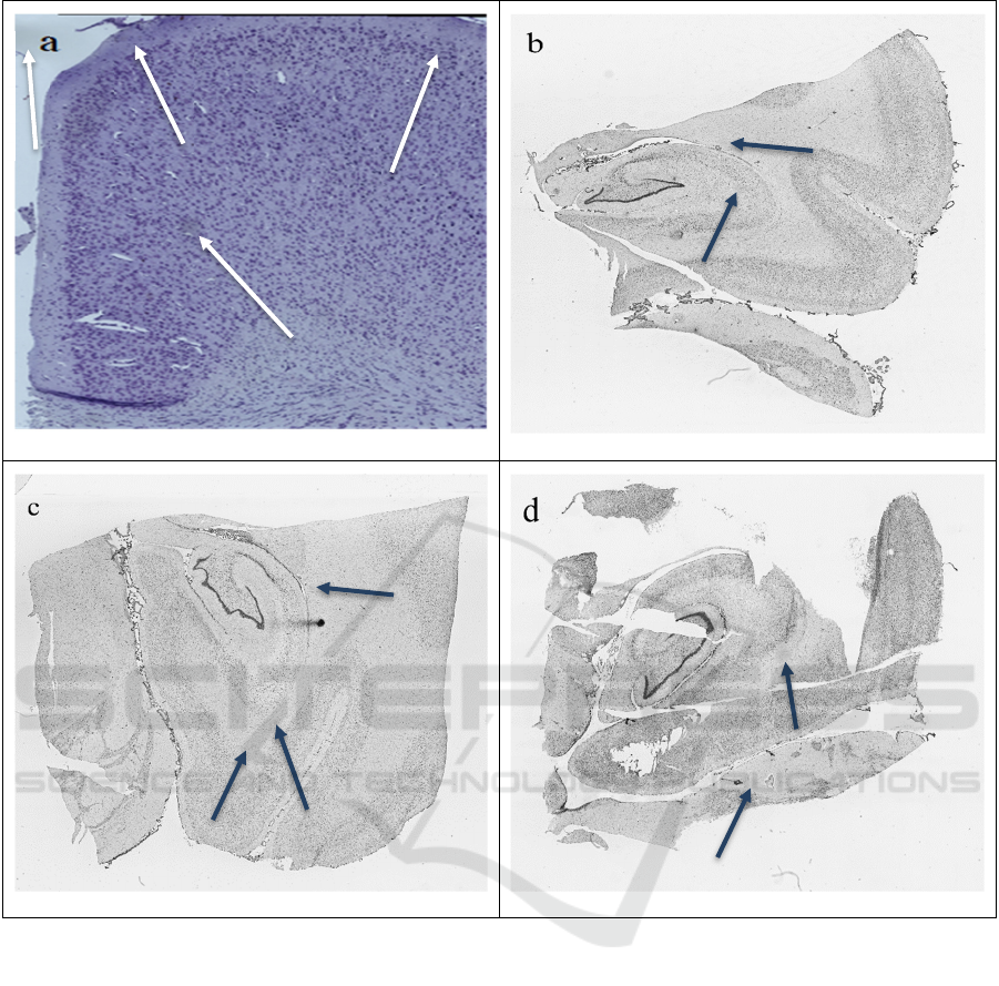
Figure 1: Examples of microscope scans with actual (arrowheads in a) and synthetically generated (arrowheads in b, c and d)

artefacts. The artefacts in b, c and d are generated using the method described in Section 2.

unevenness within the illumination field during

scanning. The centre is brighter than the peripheral

area around it (vignetting), which leads to a grid-like

structure (seams) after the reconstruction. There are

methods for removing this type of distortion;

however, they either require recording the

illumination field before the experiment or rely on

computed estimates, leading to biases and errors in

the result. Contrastingly, irregular artefacts (Figure

1a) have no method for reliable removal. They occur

due to foreign particles or defects within the optical

path, or form due to unstable tissue processing

conditions, especially in areas with non-specific

staining. These latter types are hard to predict and

treat and are thus of most interest. The outlined

innovative method for the generation of synthetic

failed microscope scans focuses on imitating them.

In this paper, we utilise Perlin Noise and Voronoi

diagrams through non-canonical means of original

use for the sake of replicating the abstract shape and

appearance of optical path artefacts in microscope

scans. Subsequently, an aptly sized dataset, consisting

of successful and unsuccessful microscope scans, can

be produced due to both algorithms’ mass versatility

and leniency (their ability to have various parameters

altered for specific desired outcomes). Generating

such a dataset is paramount. The large dataset will be

appropriate as input data to train a neural network to

remove such artefacts in natural microscope scans.

Thus, the authors have explored and identified a

BIOIMAGING 2022 - 9th International Conference on Bioimaging

118

method for realising such artificial artefacts on

microscope scans within this article. The rest of the

article is organised as follows: Section 2 outlines the

method in detail, Section 3 focuses on the results and

their outcome, Section 4 highlights the technique’s

versatility and leniency, and Section 5 discusses the

results’ implications. A note of caution, in the

subsequent paragraphs, a “cell” should be understood

as “Voronoi cell” and not the biological entity.

2 METHOD

2.1 Voronoi Generation Mixed with

Perlin Noise

Perlin noise and Voronoi diagrams have previously

been used in parallel for achieving very concentrated

and desired results (e.g., generating 3D digital

phantoms of colon tissue (Svoboda, Homola &

Stejskal, 2011) and generation of infinite virtual

terrain, a common use case (Choros & Topolski,

2016)).

This step uses Voronoi diagrams, a data structure

extensively investigated in computational geometry

(Ferrero, 2011; Berg, Krevald, Overmars &

Schwarzkopf, 1997), and Perlin noise, a type of

gradient noise (Perlin, 1985; Bae, Kim, Kim, Park,

Kim, Seo & Lee, 2018), coherently to create patches

resembling image artefacts. The authors utilized

Voronoi diagrams with the Euclidean distance

calculating function. However, diverse desired results

may be achieved using other distance metrics. A few

additional parameters were deployed to aid in

increasing the variance and prospect in results: these

parameters are “noisiness”, “excluded cells”, and

“desired cell(s)”, where “noisiness” affects the

noisiness of the Voronoi diagram (higher values

results in smaller artefacts), “excluded cells” defines

what parts of the Voronoi diagram will be removed

and “desired cell(s)” defines what patch(es) will be

used as the final artificial artefact(s).

Firstly, we define the number of cells (higher

values produce better results but increase the number

of computations), their locations (which are

arbitrarily chosen) and an “excluded” value (a label

with a value between 0 and 1, can be defined twice).

The “desired cell(s)” value is defined later since

potentially the “desired cell(s)” could be excluded if

they are above, or below if “excluded cell(s)” is

defined twice, the “excluded cell(s)” value. Also, the

authors constrained the maximum and minimum

value of each Voronoi cell’s x and y coordinates to

enhance efficacy, refer to Table 1 for more

information.

Secondly, we iterate through each pixel within the

image and identify the closest points to each cell

through calculating their Euclidian distance as thus:

𝑑𝑝,𝑞  √

∑

𝑞



 𝑝











(1)

where n defines the number of dimensions, and p and

q represent the points within Euclidean space.

Moreover, the closest points for the chosen cell are

computed using the following formula:

𝑅



 𝑥 ∈𝑿 | 𝑑𝑥,𝑃



 𝑑𝑥,𝑃



 ∀ 𝑗  𝑘 (2)

such that X is a metric space with the distance

function d, (2); K is a set of indices and (Pk) k∈K is

a tuple of non-empty subsets within the space X; and

Rk, which is associated with the site Pk, is the set of

all points within X whose distance to Pk is not higher

than their distance to the remaining sites Pj Such that

j is any index that differs from k.

Thirdly, once the closest points are decided and

each Voronoi cell is calculated, we normalise each

distance value by dividing them by the maximum-

distance value, allowing the distance values to range

between 0 and 1. Following this, a “noisiness” value

is generated (the value is a floating point number and

ideally is below 2.0), then a Perlin noise value is

generated for each pixel, which then is normalised to

a value between 0 and 1 by dividing each value by 2

and adding 1.

Mathematically, Perlin noise is defined as:

𝑝



𝑥,𝑦





∑











,











, 𝑥 𝛽



𝑥, 𝑦 𝛽



𝑦 (3)

where n defines the number of wanted ‘octaves’, p(.)

represents a simple Perlin noise function defined by

Perlin (1985), 𝛾 and 𝛽 are parameters that regulate

and control the octave magnitude and noise

smoothness. The higher 𝛽 is, the less smooth is the

noise (1), refer to Table 1.

Fourthly, we combine each normalised distance

value with its respective Perlin noise value and the

noisiness value through utilisation of equation (4):

𝑓  𝑣  𝑛 ∗ 𝑝 (4)

where 𝑣 is the normalised distance value, n is the

noisiness parameter and p is the generated and

normalised Perlin noise value, refer to Table 1.

Voronoi Diagrams and Perlin Noise for Simulation of Irregular Artefacts in Microscope Scans

119

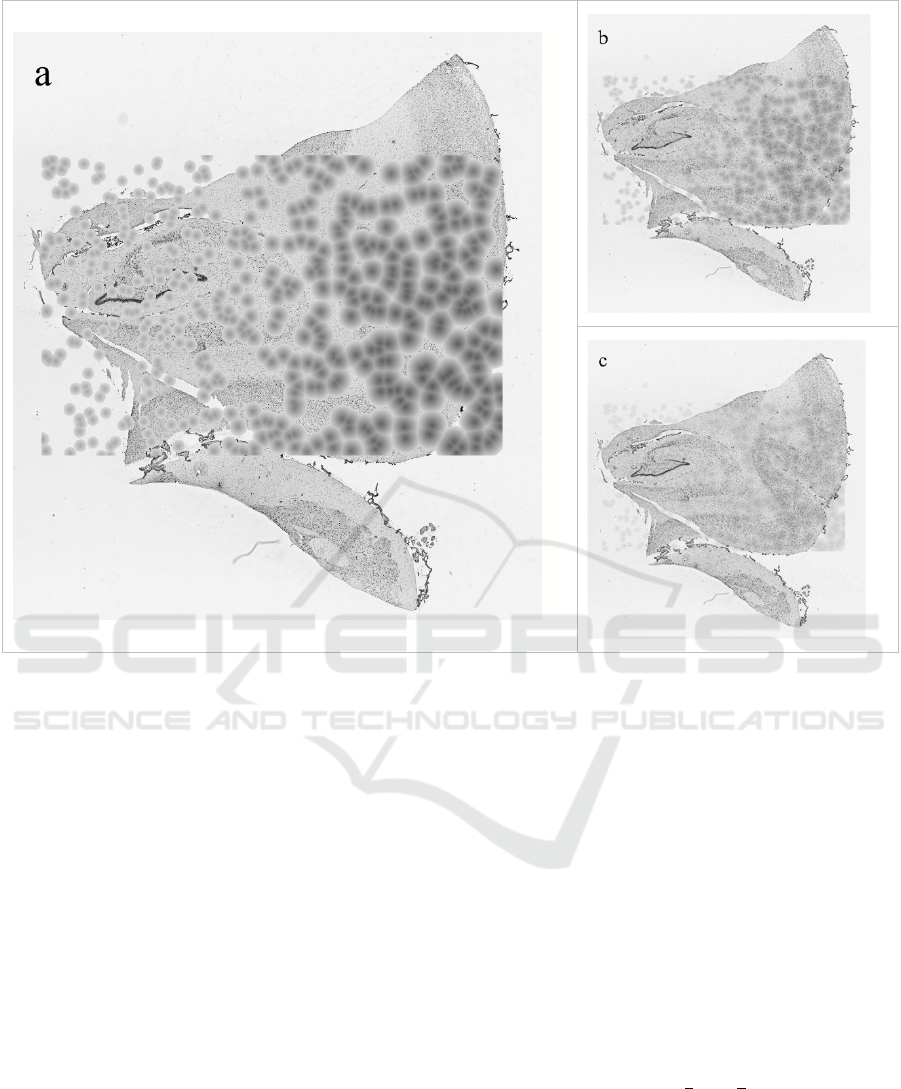
Figure 2: Examples of images produced in the intermediate steps of the algorithm: a. Result of 2.1; b. Result of 2.2; c. Result

of 2.2 after repetition.

Finally, we exclude all the undesired cells by

checking whether their final normalised value is ≥

“excluded cell(s)” (excluded if the expression

evaluates to TRUE). In this article, cells that were too

light, i.e., cells which have become non-visible and/or

do not resemble the shading of a natural artefact were

removed. The “excluded cell(s)” value allows the

programmer to control the accepted shading of their

artefact. Therefore, the criterion for estimating if a

cell is excluded can be manipulated, depending on the

desired outcome: if too light and dark artefacts are not

desired, then normalised values ≥ “excluded cell(s)”

value one and normalised values ≤ “excluded cell(s)”

value two will be excluded. Then, we multiply all the

non- removed cells’ final distance values by 255 and

set each Voronoi cell’s pixel value to the final result,

respectively. Also, a “desired cell(s)” value (which is

between 1 and the number of cells, excluding any

cells that have been removed) is generated and it will

determine what cell(s) will be used as the final

artefact(s). In the examples used in this article, the

“desired cell(s)” value was manually chosen, but it

can be assigned randomly.

2.2 Blended (Optionally Can Be

Repeated)

Within this step, we merge the original successful

microscope scan with the image generated in 2.1.

This allows an image with lighter Voronoi cells,

which fade naturally into the image to be generated.

This is essential as the periphery of actual artefacts

shows similar seamless fading into the microscope

scan. Moreover, the central color of the artefact is

lightened as well, which is vital as ideally the artefact

should not be too dark.

Both images are combined using equation (5):

𝑚



𝐴, 𝐵









𝐴





𝐵 (5)

where A represents a two-dimensional matrix of the

pixel values of the successful microscope scan, and B

represents a two-dimensional matrix of the pixel

values of the image from 2.2.

BIOIMAGING 2022 - 9th International Conference on Bioimaging

120

Table 1. Parameters used to generate the synthetic failed microscope scan demonstrated in Figure 1b.

Perlin noise n

𝜸 𝜷

scale Other parameters (Voronoi)

2.1 5 0.5 2.0

(image width,

image height)

C = 500, CL = random (x = 112-1957, y =

712-1877), EC = 0.85, DC = 183 & 186

Discretionally, this step can be repeated where the

newly blended image from this step is blended again

with the original successful microscope scan,

depending on what type of artefacts are wanted. If the

programmer wants to generate lighter artefacts that

are more subtle in appearance, then this step should

be repeated to achieve such an artefact. The authors

have repeated this step to illustrate what artefacts are

generated from such an approach (Figure 1a). Figure

1d shows artefacts from only one iteration of this step;

they are darker and more visible, generally the better

approach in most cases.

2.3 Extrapolation

Finally, for the final result generation, we use the

“desired cell(s)” parameter, defined in 2.1, to extract

the wanted cells from the image generated in 2.3 onto

the successful microscope used initially. Specifically,

this is achieved by iterating over the Voronoi section

of the image from 2.3 and checking whether it is part

of the desired cell(s). If it is, we alter the pixel value

of the original image to that of the one from 2.3. Upon

completion artefacts analogous to those in Figure 1b

are created, depending on what values were inputted

for the parameters and if 2.2 was repeated. Artefacts

in Figure 1c and 1d were generated without repetition

of 2.2.

3 RESULTS

The described algorithm generates a synthetic

artefact(s) on a successful microscope scan, as shown

in “Figure 1b and 1c”. The perceptual similarity

between both artefacts, artificial and “natural”,

pertaining to human-eye estimation, is high and

desirable: the artefacts synthetically generated within

Figure 1b, 1c and 1d naturally blend into the image

without seeming far too artificial, i.e., a massive

colour-contrast difference between the exterior of the

artefact and the pixels around it, is not present,

allowing the artefact to fade into the image and to

seem non-artificial. Also, the artefact(s) is aptly sized

and has the necessary shaping mechanism. The

method does not force the artefact(s) to be

specifically shaped; therefore, with every artefact a

somewhat abstract/realistic shape can be generated,

as seen in Figure 1b and 1c. This proves to be useful

as actual artefacts cannot be identified as having

specific shapes. Moreover, the locations and quantity

of artefacts can be controlled, meaning one successful

input image can be utilised to generate numerous

successful microscope scans with artificial artefacts.

Also, artefacts of distinctive shade can be generated

through repetition or non-repetition of step 2.2, as

seen in Figure 1b when compared to Figure 1c and

1d.

4 VERSATILITY & LENIENCY

The potency laid in a programmer’s hand regarding

achievable artefacts via the authors’ method is

immense, since the method supplies the programmer

with various parameters that can be altered for

attaining specific results, depending on what is

desired. For instance, the Perlin noise function

(Perlin, 1985) has over six parameters and directly

affects the size and shade of artefacts, enabling the

programmer to alter the respective Perlin noise

parameters to achieve lighter artefacts with smother

transitions or darker artefacts with less-smooth

transitions.

Furthermore, by manipulating the number of

Voronoi cells the programmer can alter effectively

the shape and size of the generated artefacts. The

function used for calculating the distance between

Voronoi points can be altered as numerous distance-

calculation functions exist (e.g., Euclidean (Gomathi

& Karthikeyan, 2014; Ranjitkar & Karki, 2016) and

Manhatton distance (Gomathi & Karthikeyan, 2014;

Ranjitkar & Karki, 2016)). This enables further

manipulation opportunities for the programmer; the

Voronoi Diagrams and Perlin Noise for Simulation of Irregular Artefacts in Microscope Scans

121

noisiness parameter allows to increase the roundness

of each artefact and their size, which proves to be as

artefacts vary in roundness and size.

Lastly, the parameters ‘excluded cell(s)’ and

‘desired cell(s)’ allow the programmer to deduct a

chosen proportion of cells. This controls the

generation of certain types of artefacts (lighter

artefacts, darker artefacts or artefacts of generic

shade). Visually appropriate cells can be selected

manually or automatically. The latter increases the

speed of artificial-failed microscope scan generation.

5 CONCLUSION

Within this article, the authors have described a

method for synthetic generation of “failed”

microscope scans for later use as augmented input

data within a neural network. The method outlined

within this article is promising as the generated and

the actual artefacts are very similar in visual

appearance. The artificial image distortions created

with this method naturally blend in microscope scans.

Furthermore, the method is easy to use and is

exceptionally versatile and lenient, i.e., it provides the

programmer with numerous parameters which all can

be slightly or massively tweaked to achieve

distinctive results. Finally, due to the method’s

versatility and leniency, it can synthetically generate

numerous “failed” microscope scans by only being

provided with one successful microscope scan,

allowing massive datasets to be produced for training

an artificial neural network to eliminate these

tiresome artefacts.

Although the quandaries above are intimidating to

the approach regarding restoration, the authors within

this article have developed and outlined the

foundation for solving this reoccurring and unabating

problem. The final solution will be achieved through

using a dataset generated from collecting numerous

and various successful microscope scans and their

synthetically generated failed counterparts, using the

method described within this article.

REFERENCES

Abdolhoseini, M., Kluge, M.G., Walker, F.R., & Johnson,

S.J. (2019). Neuron Image Synthesizer Via Gaussian

Mixture Model and Perlin Noise. 2019 IEEE 16th

International Symposium on Biomedical Imaging (ISBI

2019), 530-533. doi: 10.1109/ISBI.2019.8759471

Bae, H.J., Kim, C.W., Kim, N., Park, B., Kim, N., Seo,

J.B., & Lee, S.M. (2018). A Perlin Noise-Based

Augmentation Strategy for Deep Learning with Small

Data Samples of HRCT Images. Scientific Reports,

8(1). doi: 10.1038/s41598-018-36047-2

Berg, M.D., Cheong, O., Kreveld, M.V., Overmars, M., &

Schwarzkopf, O. (1997). Computational Geometry:

Algorithms and Applications. Springer-Verlag.

Choros, K., & Topolski, J. (2016). Parameterized and

Dynamic Generation of an Infinite Virtual Terrain with

Various Biomes using Extended Voronoi Diagram. J.

Univers. Comput. Sci., 22, 836-855.

Ferrero, M.M.A. (2011). Voronoi Diagram: The Generator

Recognition Problem. Computing Research Repository

- CORR.

Gomathi, V.V., & Karthikeyan, S. (2014). Performance

Analysis of Distance Measures for Computer

tomography Image Segmentation.

Peng, T., Wang, W., Rohde, G.K., & Murphy, R.F. (2009).

Instance-Based Generative Biological Shape

Modeling. Proceedings. IEEE International

Symposium on Biomedical Imaging, 5193141, 690–

693. doi: 10.1109/ISBI.2009.5193141

Perlin, K. (1985). An image synthesiser. SIGGRAPH

Comput. Graph., 19, 287-296. doi:

10.1145/325165.325247

Ranjitkar, H.S., & Karki, S. (2016). Comparison of A*,

Euclidean and Manhattan distance using Influence map

in MS. Pac-Man.

Reynolds, D. (2009). Gaussian Mixture Models. In: Li, S.Z.

& Jain, A. (eds.) Encyclopedia of Biometrics. Springer,

Boston, MA. doi: 10.1007/978-0-387-73003-5_196

Svoboda, D., Homola, O., & Stejskal, S. (2011). Generation

of 3D Digital Phantoms of Colon Tissue. In: Kamel, M.

& Campilho, A. (eds.) Image Analysis and

Recognition. ICIAR 2011. Lecture Notes in Computer

Science, 6754. Springer, Berlin, Heidelberg. doi:

10.1007/978-3-642-21596-4_4

Ulman, V., Svoboda, D., Nykter, M., Kozubek, M., &

Ruusuvuori, P. (2016). Virtual cell imaging: A review

on simulation methods employed in image cytometry.

Cytometry Part A, 89(12), 1057-1072. doi:

10.1002/cyto.a.23031

Unser, M. (1999). Splines: a perfect fit for signal and image

processing. IEEE Signal processing Magazine, 16(6),

22-38. doi: 10.1109/79.799930

Vercauteren, T., Pennec, X., Perchant, A., & Ayache, N.

(2007). Non-parametric diffeomorphic image

registration with the demons algorithm. Medical image

computing and computer-assisted intervention:

MICCAI ... International Conference on Medical Image

Computing and Computer-Assisted Intervention, 10(Pt

2), 319–326. doi: 10.1007/978-3-540-75759-7_39

Wasserman, L. (2004). All of Statistics: A Concise Course

in Statistical Inference. Springer, New York, NY. doi:

10.1007/978-0-387-21736-9

Xiong, W., Wang, Y., Ong, S.H., Lim, J.H., & Jiang, L.

(2010). Learning cell geometry models for cell image

simulation: An unbiased approach.

2010 IEEE

International Conference on Image Processing, 1897-

1900. doi: 10.1109/ICIP.2010.5652455

BIOIMAGING 2022 - 9th International Conference on Bioimaging

122