Weakly Supervised Segmentation of Histopathology Images: An Insight

in Feature Maps Ability for Learning Models Interpretation

Yanbo Feng, Adel Haﬁane and H

ene Laurent

INSA CVL, Laboratoire PRISME, Bourges, France

Keywords:

Feature Map, Convolutional Neural Network, Weakly Supervised Learning, Image Processing,

Histopathological Image.

Abstract:

Feature map is obtained from the middle layer of convolutional neural network (CNN), it carries the regional

information captured by network itself about the target of input image. This property is widely used in weakly

supervised learning to achieve target localization and segmentation. However, the traditional method of pro-

cessing feature map is often associated with the weight of output layer. In this paper, the weak correlation

between feature map and weight is discussed. We believe that it is not accurate to directly transplant the

weights of output layer to feature maps, the reason is that the global mean value of feature map loses its

spatial information, weighting scalars cannot accurately constrain the three-dimensional feature maps. We

highlight that the feature map in a speciﬁc channel has invariance to target’s location, it can stably activate the

more complete region directly related to target, that is, the feature map ability has strong correlation with the

channel.

1 INTRODUCTION

The annotation has always been a labor-intensive and

time-consuming work in deep learning. Especially for

the digital pathological image, nobody but the pathol-

ogist is able to label the image, making pixel-level

label all the more difﬁcult to obtain. Weakly super-

vised learning (WSL) (Zhou et al., 2016) has there-

fore gained lots of attention. Compared with fully-

supervised learning method, it is originally trained for

the objective of classiﬁcation using only images-level

annotation.

Since (Zhou et al., 2015) presented that convo-

lutional neural networks (CNNs) are able to carry

object information without supervision on the loca-

tion and boundary of object, most of previous studies

(Choe and Shim, 2019) (Singh and Lee, 2017) (Xue

et al., 2019) employed the feature maps outputted by

convolution layers to produce class activation maps

(CAMs) which indicate the objective area of input

image. Since the completeness and accuracy of the

target indicated in CAM is a key issue, some recent

works are undertaken to solve this problem (Bazzani

et al., 2016) (Kim et al., 2017) (Wei et al., 2017) pro-

viding better performance.

The CAM is generated by a weighted sum of fea-

ture maps. The weights from densely connected layer

are used to do the weighted sum of the outputs of

global average pooling (GAP) to generate ﬁnal scores.

The link between feature maps and weights is that the

weighted objects are the spatial average values of fea-

ture maps, so there is an assumption that the weights

can be transplanted to feature maps to calculate the

CAM of its corresponding class. However, it is not

accurate, because weights act directly on the high di-

mensional space composed of many variables, their

effects on each dimension are difﬁcult to understand.

The input variable directly acted by each weight is a

scalar, while the feature map is a three-dimensional

variable. The activation values in the feature maps

are not always directly related to the target. To bet-

ter identify the complete extent of object, high quality

feature maps need to be selected.

In this paper, based on the binary classiﬁcation

task of determining whether there is cancer in liver

pathological image, the weight distribution of fully

connected layer, the relation between feature maps

and weights, the behavior of network and the selec-

tion of high-quality feature maps are studied under

the framework of weakly supervised model. Although

CNN generates a large number of feature maps and

the processing of these feature maps is usually asso-

ciated with weights, through research, it is found that

the weights have weak correlation with the feature

Feng, Y., Haﬁane, A. and Laurent, H.

Weakly Supervised Segmentation of Histopathology Images: An Insight in Feature Maps Ability for Learning Models Interpretation.

DOI: 10.5220/0010830400003124

In Proceedings of the 17th International Joint Conference on Computer Vision, Imaging and Computer Graphics Theory and Applications (VISIGRAPP 2022) - Volume 5: VISAPP, pages

421-427

ISBN: 978-989-758-555-5; ISSN: 2184-4321

421

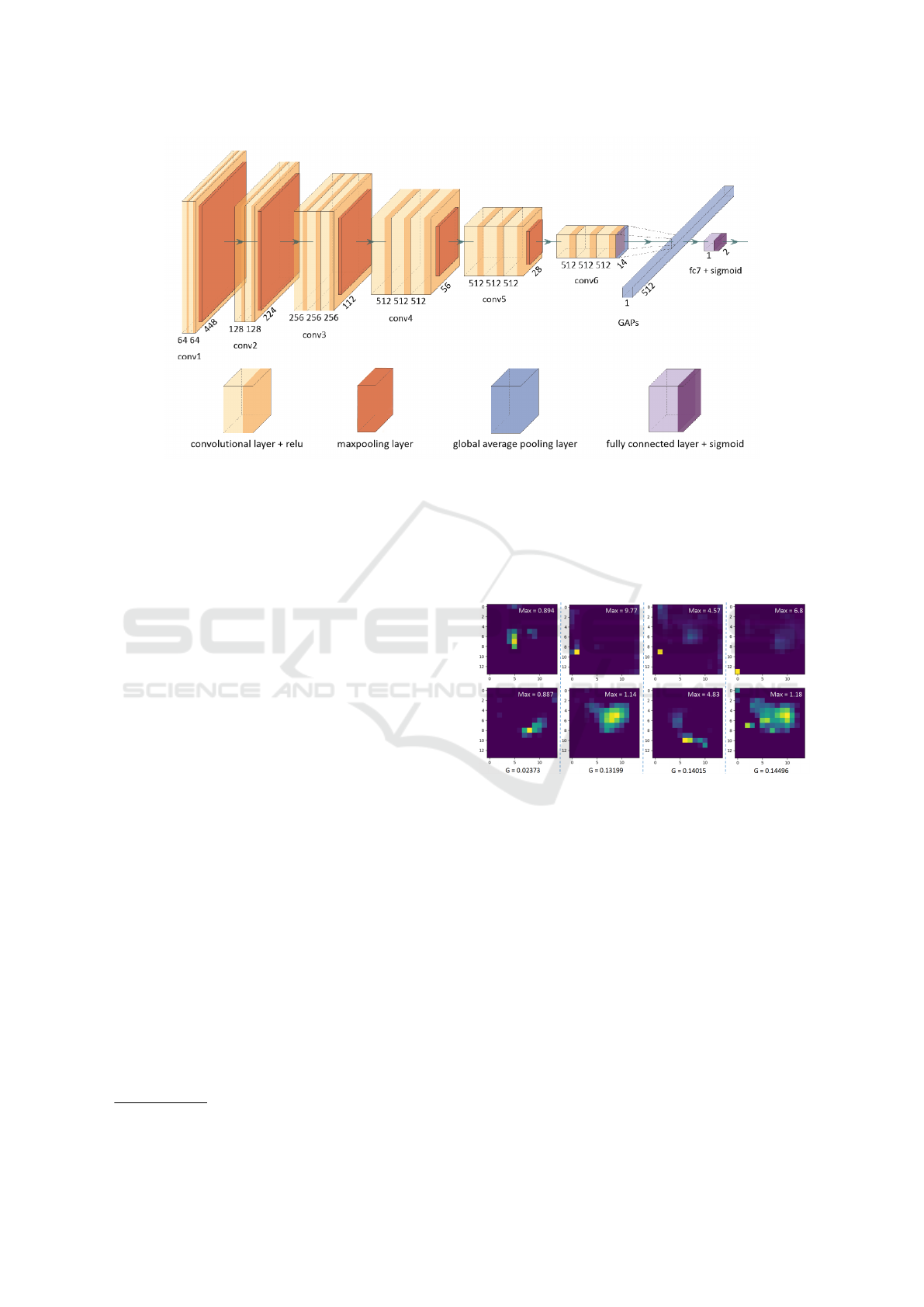
Figure 1: The architecture of weakly supervised learning model based on VGG-16.

maps and it is difﬁcult to accurately select the feature

maps directly related to target region by the weight

value. At the same time, it was found that some fea-

ture maps have the ability to activate the complete ob-

ject and are invariable to the location of target. Fur-

thermore, there exists a strong correlation between

the object-related feature maps and speciﬁc channels,

which is instructive for the purpose of feature map se-

lection.

2 METHOD AND EXPERIMENT

2.1 Dataset

The dataset used in this research comes from the 2019

MICCAI PAIP Challenge

. The original dataset con-

tains 50 WSIs and ground truths for training, 10 WSIs

and ground truths for validation, 40 WSIs for test.

All WSIs were stained by hematoxylin and eosin and

scanned by Aperio AT2 at x20 200 power. The dataset

used for WSL in this research consists of the patches

cropped from WSIs with the size of 448 x 448 pixels,

the pixel-level and patch-level labels of each cropped

image are kept for further experiments.

2.2 Conﬁguration of Model

As shown in Fig. 1, VGG-16 (Simonyan and Zisser-

man, 2014) was adopted in this study to achieve the

WSL. It could be observed that the main architecture

is maintained as original, but global average pooling

layer is used to replace the maxpooling layer and ﬂat-

https://paip2019.grand-challenge.org/dataset/

ten layer, and a densely connected layer composed of

2 elements is used as output layer using Sigmoid as

activation function.

2.3 Global Average Pooling (GAP)

Figure 2: Examples of feature maps with same GAP pre-

sented in column direction. G indicates the GAP value of

that column, Max in images indicates the maximum pixel’s

value of that image.

GAP uses a scalar, which is the average of all the

pixels of feature map to represent it, thus forms an ap-

proximate fully connected layer that can be directly

connected to the output layer. The outputted GAPs

represent the degree to which the feature maps are ac-

tivated, and all spatial information is lost. However,

a feature map has a three-dimensional space, which

consists of the two-dimensional space of pixels and

the pixels’ values. Feature maps are able to indicate

the location, the size and the boundary of object, but

GAPs can not carry these information. As shown in

Fig. 2 on several examples, two feature maps with

same GAP value can correspond to two totally differ-

ent maps.

VISAPP 2022 - 17th International Conference on Computer Vision Theory and Applications

422

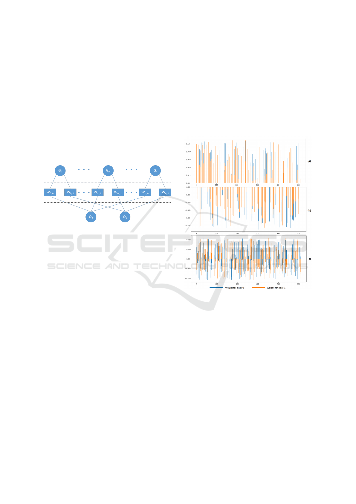
2.4 Weights in Fully Connected Layer

Fig. 3 shows the structure of the fully connected layer

of model. The weights of this layer directly process

GAPs, meanwhile they are also employed to process

their corresponding feature maps. Each GAP value

has two weights corresponding to class-0 and class-

1, which means that the same GAP value will con-

tribute to the two output units respectively after pro-

cessed by two weights. In the following discussion, it

will be mentioned that the contribution of each GAP

to each output unit will be different by adjusting the

weight. Totally there are 512 GAPs, 1024 weights

and 2 classes, namely: this is a cancer image or this is

not a cancer image.

Figure 3: The fully connected layer of the model in this

research. G

represent the GAP values, in this research n

equals 512. W represent the weights. O represent the output

elements corresponding to the 2 classes.

Based on the above structure and constituent el-

ements, the function of the fully connected layer is

realized by the weighted sum of the input variables.

Actually, the weights are ﬁxed after training, the only

variables are GAPs, as described in Eq. 1:

= Sigmoid(

∑

i=0

(i,c)

GAP(F

) +bias) (1)

where S

is the predicted score for class-c; F

is the

feature map; W

(i,c)

is the weight of i

feature map

for class-c. After weighted sum, the classiﬁcation of

input image is realized by comparing S

and S

. The

rule is that the input image belongs to the category

with the larger value. Therefore, it can be found that

the same set of feature maps will produce different

predicted values on output units to classify the input

image. The corresponding weights are the key point

in this numerical mapping.

2.5 The Numerical Relation of Weights

and the Category of Feature Maps

The weights of the full connection layer are difﬁcult

to interpret, not only because of the large number of

weights, but also the difference in value and sign. As

shown in Fig. 4 (a), (b) and (c), there are 115 GAPs

with two positive weights, 108 GAPs with two neg-

ative weights, 289 GAPs with two weights of oppo-

site signs. Among these last 289 GAPs, there are 150

positive weights for class-0, and 139 positive weights

for class-1. It should be noticed that all the outputs

of GAPs are positive, because feature maps are out-

putted by convolutional block and the Relu layer ﬁl-

ters out the negative values, thus the averages are al-

ways positive.

Figure 4: The weights for class-0 and class-1. (a) 115 same

positive weights. (b) 108 same negative weights. (c) 289

weights with opposite sign.

It can be inferred that the sign of weight deter-

mines whether the corresponding GAP increases or

decreases the predicted value, and the value of weight

determines how much the GAP contributes to the pre-

dicted value. Fig. 4 (a) and (b) show that even the

weights have same sign, their values are different,

which means that GAPs will contribute to the ﬁnal

predicted scores differently. While the weights with

opposite sign mean that the same GAP could increase

the ﬁnal predicted score of one class, at the same time,

it will reduce the one of another class. The weights

are ﬁxed after training, the sign and numerical dif-

ferences of weights could be the difference of GAPs,

furthermore be the category of feature maps.

Based on the above observation, the numerical re-

lation between weights belonging to two categories of

the same GAP may carry category information about

Weakly Supervised Segmentation of Histopathology Images: An Insight in Feature Maps Ability for Learning Models Interpretation

423

the feature map. In addition, based on Eq. 1, it is

logical to make the assumption that the feature maps

related to corresponding class will be given a lager

weight of that class for the sake of improving the pre-

dicted score. Thus, it is found that the feature map

can be classiﬁed by comparing the weights belonging

to two output units of its corresponding GAP. The

rule of classiﬁcation is that the feature map belongs

to the class with the larger weight value. As shown

in Fig. 5, the feature maps of three images are ﬁrstly

classiﬁed according to the above rules, and then the

location of the maximum pixel in each feature map is

selected for drawing.

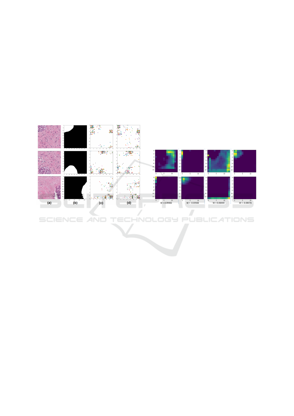
Figure 5: Three examples of classifying feature maps by

weights. (a) original input images. (b) ground truths. (c) the

maximum value graph of class-1. (d) the maximum value

graph of class-0.

Through comparison, it is found that relatively

more points fall within the cancer area in the graph

belonging to class-1, relatively more points fall within

the normal tissue area in the graph belonging to class-

0. This observation supports the above hypothesis to a

certain extent, the numerical relationship between two

weights of the same GAP value is related to the clas-

siﬁcation of corresponding feature graphs. However,

this method cannot classify the feature map exactly,

it can be observed from Fig. 5 that there are points

that don’t belong to the appropriate categories respec-

tively concerned by class-1 and class-0. Applying this

method to classiﬁcation can only achieve a fuzzy clas-

siﬁcation effect, that is, the number of correct points

is higher than the number of wrong points. This re-

sult also proves that the weight is originally weakly

representative of the feature map.

2.6 Correlation between Feature Maps

with Same Weight Value

On the basis of the previous section, the weak rela-

tionship between feature maps and weights is further

explained through experiments in this section. As

shown in Fig. 6, there are four pairs of feature maps

with same weight value for a given class. It can be ob-

served that the activated regions in each feature map

vary greatly. The activated regions in the feature map

have different features, some are continuous pixels,

some are scattered pixels, and some do not output ac-

tivated pixels. Several feature maps have overlapping

areas, such as the 2

and 3

columns, and their cross

areas are relatively small. Therefore, the correlation

between feature maps is low even though they have

the same weight values.

Figure 6: Examples of feature map with same weight. The

two images in each column have same weight value, W

represents the value of weight with the margin of error

±0.00001.

To prove this point further another experiment is

done in this research. 12 pairs of approximately equal

weights are chosen, their corresponding feature maps

are ﬁrstly binarilized by Otsu’s method and then eval-

uated by F1 score. 8000 images are tested, the average

F1 scores are shown in Table. I. According to the data

listed in the table, the activated regions in each pair of

feature maps have almost no correlation. This result

further proves that the value of weight does not repre-

sent the activated features of feature maps, the feature

map has no close relation with the value and the sign

of weight.

2.7 Feature Map Integrity and Speciﬁc

Channels

As can be seen from the previous sections, it is difﬁ-

cult to ﬁnd feature maps directly related to the target

through weights. In addition to the above reasons, an-

other one is that many feature maps do not activate

the complete target region, and most of them have

scattered irregular pixels. Actually, the weights of

VISAPP 2022 - 17th International Conference on Computer Vision Theory and Applications

424

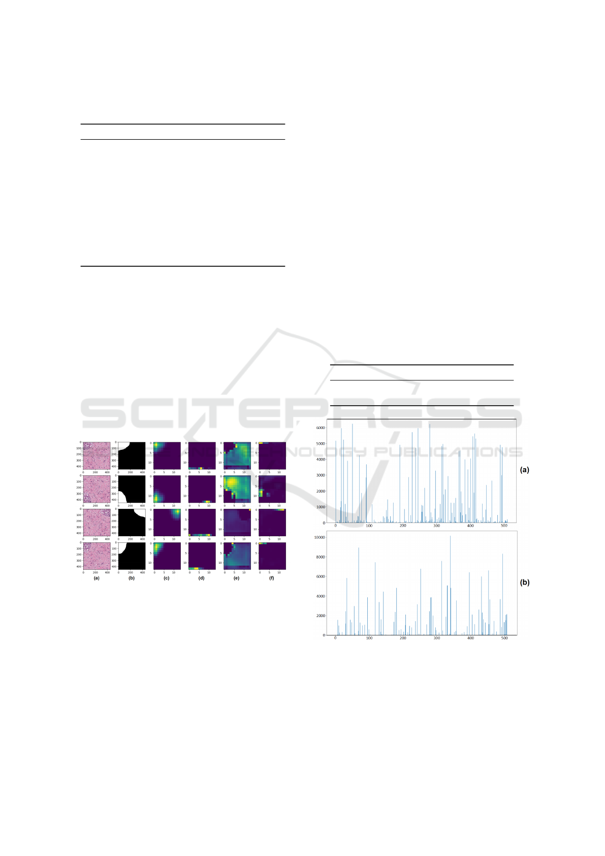
Table 1: The result of experiment to test the similarity of

feature maps with relatively equal weights.

Channels Weight (±0.00001) F1 score

16 & 167 0.08313 0.00000e+00

21 & 477 0.10225 0.00000e+00

43 & 374 -0.07273 0.00000e+00

47 & 362 -0.05665 0.00000e+00

49 & 50 0.09689 0.00000e+00

56 & 252 -0.06634 0.00000e+00

69 & 256 -0.03166 2.70269e-06

104 & 154 -0.05188 0.00000e+00

124 & 383 0.08003 0.00000e+00

164 & 308 0.07023 1.00540e-04

276 & 312 0.00364 0.00000e+00

329 & 481 0.00089 0.00000e+00

output layer are ﬁxed after training, beyond the nu-

merical level of the weights, the channel in which the

GAP is located is another potentially valuable obser-

vation point. The activated area in feature maps is not

ﬁxed, it changes with the changes of region of interest

(ROI). From this point of view the numerical relation-

ship between weights and GAP is not solid. Weights

are more inclined to a structural distribution in order

to achieve the overall effect, which is speciﬁc in this

study. The channel is indeed related to the feature.

Namely some feature maps in ﬁxed channels are able

to capture class-1 and class-0 information. Fig. 7 il-

lustrates this point, four feature map are chosen to be

visualized.

Figure 7: Each column from left to right present (a) in-

put images, (b) ground truths, (c) 51

feature maps, (d)

feature maps, (e) 69

feature maps and (f) 70

fea-

ture maps.

It is observed that not all of the feature maps ac-

tivate the ROI partially or scatteredly, some of them

present the ROI relatively completely compared with

the ground truth. Among the four channels chosen to

be visualized in Fig. 7, 51

and 69

feature maps

activate the areas directly related to cancer area and

normal tissue area. Actually, not only the object of

cancer area, but also the normal tissue area is taken

as object for the network. 51

and 69

position are

chosen particularly to prove that these single feature

maps in ﬁxed position have the ability to capture the

whole object and are shift-invariant for object. 52

and 70

feature maps are chosen randomly showing

that some feature maps capture the features that have

low comprehensibility. Furthermore, several images

have been tested to check the reproducibility of this

idea. Here, 8000 images are tested to verify the re-

lation between 51

, 52

, 69

and 70

feature maps

and their ground truths. Otsu’s method is used to seg-

ment the feature maps ﬁrstly, then the similarity be-

tween the binarilized image and their ground truth is

evaluated by F1 score. The result is shown in Table II,

it can be observed that 51

and 69

feature maps are

strongly correlated with cancer area and normal tissue

area respectively in contrast with 52

and 70

fea-

ture maps which consistently output image data that

has nothing to do with target areas.

Table 2: The result of experiment to test the similarity be-

tween feature maps in ﬁxed position and corresponding ob-

ject.

Channel F1 score Channel F1 score

51 0.54401 69 0.59972

52 0.00837 70 0.04147

Figure 8: The result of selecting feature maps. (a) the fea-

ture maps directly related to class-1, (b) the feature maps

directly related to class-0. The X-axis is channel position,

and the Y-axis is cumulative score.

Not only 51

and 69

feature maps are able to

present the complete area of target, there are more fea-

ture maps that activate the area directly related to can-

Weakly Supervised Segmentation of Histopathology Images: An Insight in Feature Maps Ability for Learning Models Interpretation

425

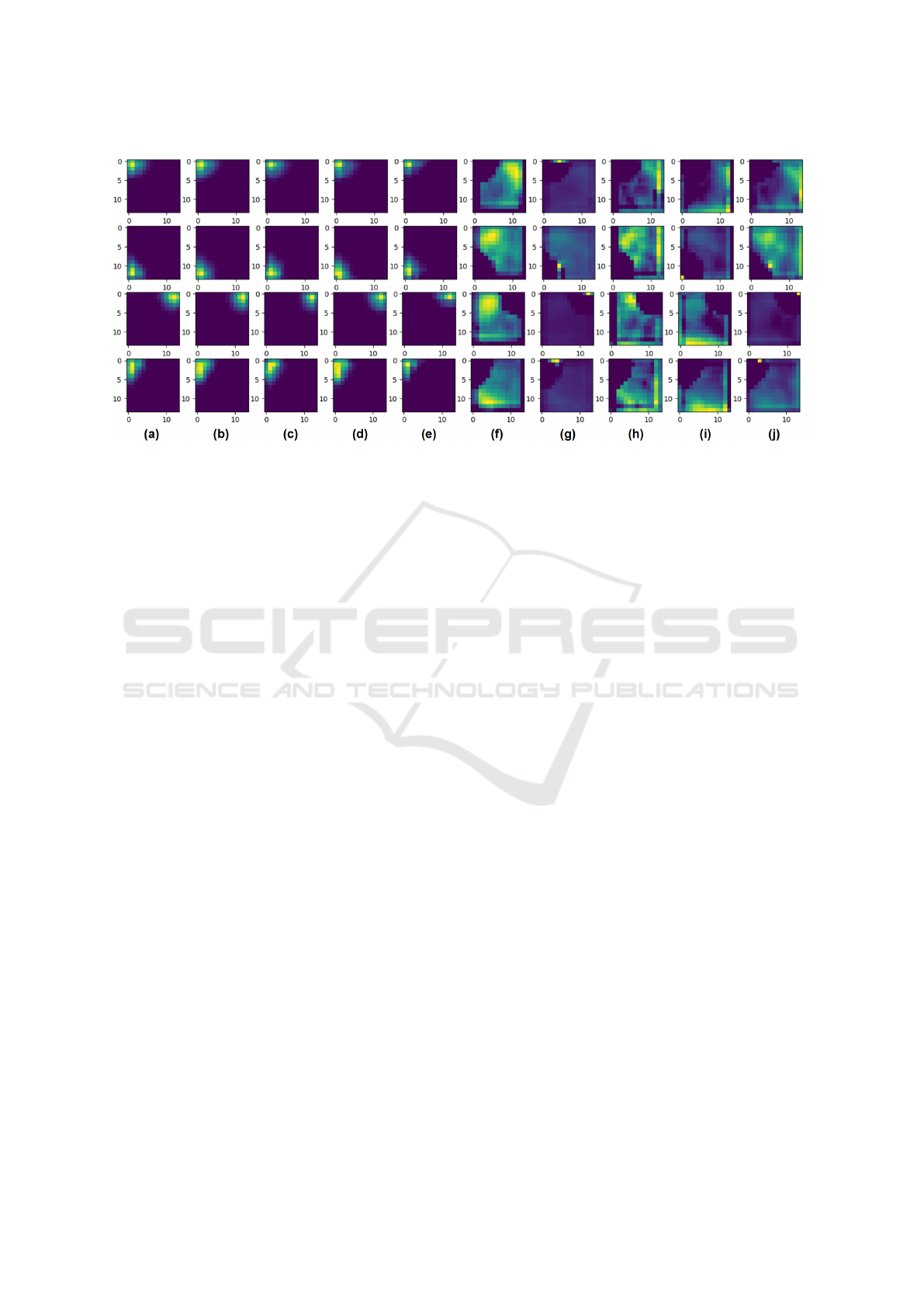
Figure 9: Each column from left to right is (a) 1

, (b) 18

, (c) 191

, (d) 228

, (e) 245

, (f) 118

, (g) 314

, (h) 327

, (i)

331

, (j) 432

channel.

cerous and normal tissues. As shown in Fig. 9, there

are ten channels that are able to capture the whole ob-

ject information for the four original images in Fig.

7. Furthermore, 16000 images are used to select out

the channels that reﬂect the relatively complete tar-

get area in this research. The 512 feature maps of

each image are once again ﬁrstly segmented by Otsu’s

method, then the similarity between the binarilized

images and the ground truth is evaluated by F1 score.

If the score is larger than 0.6, that position gets score

1. Fig. 8 presents the cumulative score obtained by

each of the 512 channels over the 16000 images. It

can be observed in the ﬁnal results that there are spe-

ciﬁc channels among the 512 channels that continu-

ously capture feature areas associated with the can-

cerous and normal tissues. This result demonstrates

that the ability of feature maps to activate the com-

plete regions directly related to the target is tied to

particular channels.

3 DISCUSSION

The CNN produces a great number of feature maps

in the middle layers. Since these feature maps are

captured by the network itself, a large part of them

are not able to directly activate the complete target

region, and some of them are unreadable from the hu-

man point of view and irrelevant to the target. Mean-

while, there are feature maps that reﬂect relatively

complete target area. The complete extent of object

is the key point in weakly supervised learning for the

tasks of segmentation and localization. If the feature

maps with complete activated regions directly related

to the target can be selected from numerous feature

maps, the accuracy of subsequent processing will po-

tentially be improved.

The trained model has ﬁxed weight for each fea-

ture map. It was expected to extract the feature map

with complete target area based on these weights, but

the experiments above have proven that it is inaccu-

rate. In addition to the reasons presented in Section

2. 5 and Section 2. 6, the randomness of the GAPs

with same values also indicates the inefﬁciency of the

weight’s dependence on the values of GAPs. Since

GAPs are the spatial average of feature map, same

GAPs emerge randomly with the position and size of

the target changing, but their weights are discrimina-

tive. The same scalar values are treated with different

weights, this suggests that the difference is due to the

channel.

The classiﬁcation of feature map realized by com-

paring the weights of two classes numerically is not

accurate. Note that a phenomenon appeared in the

observation and analysis of 512 feature maps and 512

pairs of weights that, among the two weights of a

feature map related to class-1, the weight belonging

to class-0 category is sometimes larger. This phe-

nomenon means that the feature map related to class-

1 will contribute more to class-0. The opposite case

also exists, which is also reﬂected in the points that

are misclassiﬁed in Fig. 5. However, it can be ob-

served in Fig. 5 that the number of misclassiﬁed

points is relatively small compared to the number of

correctly classiﬁed points. The reason could be ex-

plained by the stability of high dimensional systems,

since the original processing object of weights is a

high-dimensional space made up of 512 scalars. It is

not the features belonging to a single class that deter-

VISAPP 2022 - 17th International Conference on Computer Vision Theory and Applications

426

mine the ﬁnal classiﬁcation, which makes the system

robust. From this point of view, the method of classi-

fying feature maps using numerical relationships be-

tween weights is inherently ﬂawed. The numerical

relationship of weights can not clearly represent the

category of feature maps.

The ability to activate complete target regions of

feature maps is found in ﬁxed channels. This prop-

erty of neural networks applies to both cancerous and

normal tissue areas, treating both classes as targets

and activating the corresponding area completely. At

the same time, speciﬁc channels are invariant to tar-

get changes in the input image, they can stably output

the complete active area. In addition, this capability is

closely tied to channels from which feature maps can

be obtained once the channels are identiﬁed. There-

fore, after the training of neural network, the channels

can be screened with a small amount of data to deter-

mine the needed channels.

4 CONCLUSION

In this paper, we have taken an insight into the neu-

ral network. we have explained the weak correlation

between feature map and the weight of output layer.

The feature map directly related to target cannot be

selected out through the numerical characteristics of

weights. It was also found that the feature map in

speciﬁc channel has the ability to capture ﬁxed fea-

ture. The conducted experiments prove that the fea-

ture maps which activate the more complete target re-

gion are output in ﬁxed channels. This work can aid

other researchers in understanding and designing net-

works for image processing.

ACKNOWLEDGEMENTS

The authors gratelfully acknowledge ﬁnancial support

from China Scholarship Council.

REFERENCES

Bazzani, L., Bergamo, A., Anguelov, D., and Torresani, L.

(2016). Self-taught object localization with deep net-

works. In 2016 IEEE Winter Conference on Applica-

tions of Computer Vision (WACV), pages 1–9.

Choe, J. and Shim, H. (2019). Attention-based dropout

layer for weakly supervised object localization. In

2019 IEEE/CVF Conference on Computer Vision and

Pattern Recognition (CVPR), pages 2214–2223.

Kim, D., Cho, D., Yoo, D., and Kweon, I. S. (2017). Two-

phase learning for weakly supervised object localiza-

tion. In 2017 IEEE International Conference on Com-

puter Vision (ICCV), pages 3554–3563.

Simonyan, K. and Zisserman, A. (2014). Very Deep Con-

volutional Networks for Large-Scale Image Recogni-

tion. arXiv e-prints, page arXiv:1409.1556.

Singh, K. K. and Lee, Y. J. (2017). Hide-and-seek: Forc-

ing a network to be meticulous for weakly-supervised

object and action localization. In 2017 IEEE Interna-

tional Conference on Computer Vision (ICCV), pages

3544–3553.

Wei, Y., Feng, J., Liang, X., Cheng, M.-M., Zhao, Y., and

Yan, S. (2017). Object region mining with adversarial

erasing: A simple classiﬁcation to semantic segmen-

tation approach. In 2017 IEEE Conference on Com-

puter Vision and Pattern Recognition (CVPR), pages

6488–6496.

Xue, H., Liu, C., Wan, F., Jiao, J., Ji, X., and Ye, Q. (2019).

Danet: Divergent activation for weakly supervised ob-

ject localization. In 2019 IEEE/CVF International

Conference on Computer Vision (ICCV), pages 6588–

6597.

Zhou, B., Khosla, A., Lapedriza, A., Oliva, A., and Tor-

ralba, A. (2016). Learning deep features for discrimi-

native localization. In 2016 IEEE Conference on Com-

puter Vision and Pattern Recognition (CVPR), pages

2921–2929.

Zhou, B., Khosla, A., Lapedriza, g., Oliva, A., and Tor-

ralba, A. (2015). Object detectors emerge in deep

scene cnns. In International Conference on Learning

Representations.

Weakly Supervised Segmentation of Histopathology Images: An Insight in Feature Maps Ability for Learning Models Interpretation

427