On Solving the Minimum Common String Partition Problem by Decision
Diagrams
Milo
ˇ
s Chrom
´
y
a
and Markus Sinnl
b
Institute of Production and Logistics Management/JKU Business School, Johannes Kepler University Linz, Altenberger
Straße 69, 4040 Linz, Austria
Keywords:
Decision Diagram, Bioinformatics, Computational Biology, Minimum Common String Partition Problem.
Abstract:
In the Minimum Common String Partition Problem (MCSP), we are given two strings on input, and we want
to partition both into the same collection of substrings, minimizing the number of the substrings in the par-
tition. This combinatorial optimization problem has applications in computational biology and is NP-hard.
Many different heuristic and exact methods exist for this problem, such as a Greedy approach, Ant Colony
Optimization, or Integer Linear Programming. In this paper, we formulate the MCSP as a Dynamic Program
and develop an exact solution algorithm based on Decision Diagrams for it. We also introduce a restricted
Decision Diagram that allows to compute heuristic solutions to the MCSP and compare the quality of solution
and runtime on instances from literature with existing approaches. Our approach scales well and is suitable
for heuristic solutions of large-scale instances.
1 INTRODUCTION
A string is a sequence of symbols such as letters of the
English alphabet, numbers, or nucleotides (ACGT)
forming a DNA sequence. Many optimization prob-
lems related to strings are widespread in bioinformat-
ics, such as the Far-from Most String Problem (Mene-
ses et al., 2005; Mousavi et al., 2012), the Longest
Common Subsequence Problem and its variants (Hsu
and Du, 1984; Smith and Waterman, 1981), and Se-
quence Alignment Problems (Gusfield, 1997). In this
paper we focus on the Minimum Common String Par-
tition Problem (MCSP). In the MCSP we are given
two or more related input strings, where related means
they contain the same symbols. A solution is the par-
titioning of each input string into the same collection
of substrings. The objective is to minimize the size of
the obtained collection.
Example 1. Consider the MCSP on two DNA se-
quences s
1
= GAGACTA and s
2
= AACTGAG. Ob-
viously, s
1
and s
2
are related because A appears three
times in both input strings, G appears twice in both
input strings, and C and T appear only once. A
trivial valid solution can be obtained by partition-
ing both strings into substrings of length one P
1
=
a
https://orcid.org/0000-0002-5357-1304
b
https://orcid.org/0000-0003-1439-8702
P
2
= {A,A,A,C,T,G, G}. The objective function
value of this solution is 7. However, the optimal so-
lution with objective function value 3 is P
1
= P
2
=
{A,ACT,GAG}.
The MCSP is closely related to the Problem of
Sorting by Reversals with Duplicates, a key problem
in genome rearrangement (Chen et al., 2005).
The work of (Goldstein et al., 2005) proved the
NP-hardness of the MCSP. Different heuristics for
the MCSP were introduced, such as a Greedy ap-
proach (Chrobak et al., 2004; He, 2007), Proba-
bilistic Tree Search (TRESEA) (Blum et al., 2014),
Ant Colony Optimization (ACO) (Ferdous and Rah-
man, 2017). Moreover, also various exact approaches
based on Integer Linear Programming (ILP) mod-
els (Blum, 2020; Blum et al., 2015; Blum et al., 2016;
Blum and Raidl, 2016) were proposed.
Our Contribution. In this work, we develop a Deci-
sion Diagram (DD) approach to the MCSP.
A DD can be used for computing the exact so-
lution of a chosen optimization problem. However,
NP-hard problems such as the MCSP could have an
exponentially large DD representation. By relax-
ing and restricting DDs, lower and upper bounds for
the objective function value of a optimization prob-
lem can be obtained (Bergman et al., 2016). Such
DD approaches were already used for various com-
binatorial problems such as Graph Coloring, Maxi-
Chromý, M. and Sinnl, M.
On Solving the Minimum Common String Partition Problem by Decision Diagrams.
DOI: 10.5220/0010830200003117
In Proceedings of the 11th International Conference on Operations Research and Enterprise Systems (ICORES 2022), pages 177-184
ISBN: 978-989-758-548-7; ISSN: 2184-4372
Copyright
c
 2022 by SCITEPRESS – Science and Technology Publications, Lda. All rights reserved
177

mal Independent Set, MaxSAT (Bergman et al., 2016;
van Hoeve, 2020), and various sequence and string
problems such as Repetition-Free Longest Common
Subsequence (Horn et al., 2020), Multiple Sequence
Alignment (Hosseininasab and van Hoeve, 2021), or
Constraint-Based Sequential Patter Mining (Hossein-
inasab et al., 2019). DDs are also suitable for a hybrid
approach with ILP solvers combined using Machine
Learning methods (Gonz
´
alez et al., 2020; Tjandraat-
madja, 2018).
This paper introduces an exact and a restricted
DD for the MCSP. We compare their performance
for solving the MCSP with existing results achieved
by ACO, TRESEA, and ILP models on the dataset
used in (Blum et al., 2015), (Blum et al., 2014; Blum
et al., 2016) and (Ferdous and Rahman, 2017).
Our goal is to motivate further research by com-
paring the DD approach with existing heuristic ap-
proaches for the MCSP. We show that our restricted
DD allows computation of better objective function
values than ACO (Ferdous and Rahman, 2017) for
most instances, and better objective function values
than TRESEA (Blum et al., 2014) for large instances.
Moreover, we show that our restricted DD approach
is much faster than any of the currently applied meth-
ods (ACO, TRESEA, ILP (Blum et al., 2015; Blum
et al., 2014; Blum et al., 2016; Blum and Raidl, 2016;
Ferdous and Rahman, 2017)).
Outline of the Paper. The paper is organized as fol-
lows. In the Section 2, we go through basic definitions
used in the paper. In Section 3, we introduce a Dy-
namic Program (DP) formulation of the MCSP. This
formulation allows us to define exact and restricted
DDs for the MCSP, which we also do in this section.
We describe the main implementation details in the
Section 3. In Section 4, we present our experimental
results, and in the last Section 5, we summarize the
results and set up goals for future research.
2 DEFINITIONS
First, we define a notion of a Minimization Prob-
lem, the Dynamic Program and Decision Diagram
for a Minimization Problem, following the defini-
tions given in (Bergman et al., 2016; Tjandraatmadja,
2018). Finally, we also formally define the Minimum
Common String Partition Problem.
Minimization Problem. We consider the Boolean
Minimization Problem P over n Boolean variables,
where we try to minimize the function value f (x)
according to the constraints C
i
(x), i = 1,. .., m and
x ∈ {0,1}
n
. Constraints C
i
(x) state an arbitrary re-
lation between two or more variables. A feasible so-
lution to P is an assignment x ∈ {0, 1}
n
satisfying all
constraint C
i
(x), i = 1, ... ,m. The set Sol(P) is the
set of all feasible solutions to P. A feasible solution
x
∗
∈ Sol(P) is optimal for P if f (x
∗
) ≤ f (x) for all
x ∈ Sol(P). The set Opt(P) is the set of all optimal
solutions of problem P.
Dynamic Program. A Dynamic Program (DP) for a
given problem P with n Boolean variables consists of
a state space S with n + 1 stages, a partial transition
function t
j
, and a transition cost function h
j
.
• The state space S is partitioned into sets for each
of the n + 1 stages; i.e., S is the union of the sets
S
0
,. .., S
n
, where S
0
contains only the root state ˆr,
and S
n
contains only the terminal state
ˆ
t.
• The partial transition functions t
j
defines how
the decisions govern the transition between states.
Note that this functions is not necessarily defined
for each state and decision, however each state has
defined a transition for at least one decision.
• The transition cost functions h
j
is defined for each
transition defined by t
j
and gives the cost for tak-
ing this transition. To account for objective func-
tion constants, we also consider a root value v
r
which is constant that will be added to the transi-
tion costs directed out of the root state.
The DP formulation has variables (s,x) = (ˆr =
s
0
,. .., s
n
=
ˆ
t,x
0
,. .., x
n−1
). The objective function
value we try to minimize is
ˆ
f = v
r
+
∑
n−1
j=0
h
j
(s
j
,x
j
)
with s
j+1
= t
j
(s
j
,x
j
) s
j
∈ S
j
, j = 0,. .., n − 1 for a
defined transition function t
j
.
This formulation is valid for a problem P if, for
every x ∈ Sol(P) there is an s ∈ S
0
×S
1
×. ..×S
n
such
that (s,x) is feasible and
ˆ
f (s, x) = f (x).
Decision Diagrams. A Decision Diagram (DD) D =
(U,A, h) is a arc-weighted layered directed acyclic
multigraph with node set U , arc set A, weight func-
tion h : A → R, and arc labels 0 and 1. The node
set is partitioned into layers L
0
,. .., L
n
, where layer
L
0
contains only root node r and L
n
contains only
terminal T. The width of the layer is the number
of the nodes it contains. We also consider a weight
v
r
∈ R of the root node r for problem specific con-
stants. Each node on layer L
j
is associated with a
Boolean variable x
j
. Each arc a ∈ A is directed from
a node n
j
∈ L
j
to a node n
j+1
in the next layer L
j+1
and has a label 0 for a 0-arc or 1 for 1-arc that rep-
resents assignment a value 0 or 1 to a variable x
j
.
The node n
j
[x
j
= 0] denotes the endnode of the 0-
arc with a start node n
j
, and the node n
j
[x
j
= 1] de-
notes the endnode of 1-arc with a start node n
j
. Every
arc-specified path p = (a
0
,a
1
,. .., a
n−1
) from r to T
encodes an assignment to the variables x
0
,. .., x
n−1
,
namely x
j
= a
j
, j = 0,. .., n − 1. The weight of such
ICORES 2022 - 11th International Conference on Operations Research and Enterprise Systems
178

path is h(p) = v
r
+
∑
n−1
j=0
h(a
j
). The set of r-T paths of
D represents the set of assignments Sol(D). The set
of all minimum weighted r-T paths of D represents
the set of optimal assignments Opt(D).
A DD D is exact for problem P if Sol(D) =
Sol(P). The benefit of using exact DDs for represent-
ing solutions is that equivalent nodes, i.e. nodes with
the same set of completions, can be merged. A DD is
called reduced if no two nodes in a layer are equiva-
lent. A key property is that for a given fixed variable
ordering, there exists a unique reduced DD. Nonethe-
less, even reduced DDs may be exponentially large to
represent all solutions for a given problem.
A DD D is restricted for problem P if Sol(D) ⊆
Sol(P) and h(x
∗
D
) ≥ f (x
∗
P
) for x
∗
D
∈ Opt(D) and x
∗
P
∈
Opt(P). Such a restricted DD can give us a heuristic
solution of a minimization problem in short comput-
ing time and with manageable memory requirements.
Minimum Common String Partition Problem. An
alphabet Σ = {a
1
,a
2
,. .., a
|Σ|
} is a finite set of sym-
bols. A string s is a finite sequence of symbols from
Σ. The length n of a string s is the number of symbols
in s. A substring s[i : j], 0 ≤ i < j ≤ n denotes a sub-
string of s consisting of symbols of s starting at index
i and ending on index j − 1. The term 1
k
(0
k
) denotes
a string of k repeating ones (zeroes).
Two strings s
1
,s
2
are related iff each symbol ap-
pears the same number of times in each of them. A
valid solution to the MCSP is a partitioning of s
1
and
s
2
into multisets P
1
and P
2
of non-overlapping sub-
strings, such that P
1
= P
2
. The value of the solution
to the MCSP is the size of partitioning |P
1
| = |P
2
| and
the goal is to find a solution with the minimal value.
3 MODELING THE MCSP AS DD
First, we describe the DP formulation of the MCSP.
We then use the DP formulation to describe the exact
DD formulation of the MCSP. Lastly we describe a
restricted DD for the MCSP.
3.1 MCSP as a Dynamic Program
Consider the MCSP on two related strings s
1
,s
2
of
length n. A block b
i
is a tuple (k
1
i
,k
2
i
,t
i
) such that
k
1
i
,k
2
i
∈ {0,.. .,n − t
i
}, t
i
∈ {1,.. .,n} and substrings
s
1
[k
1
i
: k
1
i
+t
i
] and s
2
[k
2
i
: k
2
i
+t
i
] are equal, i.e. contain
same symbols in same order. Two blocks b
i
, b
j
over-
lap if k
1
i
− t
j
< k
1
j
< k
1
i
+ t
i
or k
2
i
− t
j
< k
2
j
< k
2
i
+ t
i
holds. This means, that both b
i
and b
j
are associated
with at least one same position ` = {1, ... ,n} in the
input strings s
1
and s
2
. Otherwise the blocks do not
overlap.
Example 2. Consider the MCSP on two DNA se-
quences s
1
=
[
GAG
g
ACTA and s
2
= A
g
ACT
[
GAG as
in Example 1. We consider blocks b
i
= (2, 5,2) as-
sociated with the string GA, b
j
= (3,1,3) associated
with the string
g
ACT, and block b
`
= (0,4,3) asso-
ciated with the string
[
GAG. String b
i
and b
j
overlap
only at position 3 in the first string s
1
. Blocks b
i
and b
`
overlap in both strings in positions s
1
[2] and s
2
[5 : 7].
The blocks b
j
and b
`
does not overlap.
Let us define the set of all blocks of length at least
two as B with associated index set I, i.e., each index
(k
1
,k
2
,t
b
) ∈ I corresponds to a block in B.
The variables of our DP formulation of the MCSP
are indexed by the index set I
λ
= I ∪ {λ} where I is
the index set of our blocks and λ 6∈ I is a special index.
The set of variables is defined as X = {x
i
|i ∈ I
λ
}. Each
variable x
i
, i ∈ I is associated with the corresponding
block and the variable x
λ
is a variable, which is used
in the last step in the DP to indicate the covering of the
remaining uncovered symbols by blocks of size one.
The constrains of the MCSP are defined as ¬(x
i
∧ x
j
)
for each i, j such that blocks b
i
, b
j
overlap.
A state of our DP is defined by a tuple of bitsrings
(bs
1
,bs
2
), where bs
1
,bs
2
∈ {0,1}
n
. Let B
`
⊆ B be the
set of all blocks previously considered when we are in
state ` of our DP. Let bs
1
[ j] indicate the j-th position
in bs
1
. The value of bs
1
[ j] is zero if and only if the
position j in s
1
is contained in a block b
i
∈ B
`
where
we chose x
i
= 1. Similarly bs
2
[ j] = 0 if and only if
position s
2
[ j] is contained in any block b
i
∈ B
`
where
we chose x
i
= 1.
The root state is (1
n
,1
n
) as no position is yet cov-
ered and the terminal state is (0
n
,0
n
) as all positions
have to be covered in a feasible solution.
The transition function for a state (bs
1
,bs
2
) and a
variable x
i
, i ∈ I
λ
is
• (bs
1
,bs
2
) for i ∈ I, x
i
= 0, with the cost 0.
• (bs
1
new
,bs
2
new
) where c = 0,1 bs
c
new
[ j
c
] = 0 for all
k
c
i
≤ j
c
< k
c
i
+t
i
and bs
c
new
[ j
c
] = bs
c
[ j
c
] otherwise.
The cost of this transition is 1 − t
i
. This transi-
tion is defined only if i ∈ I, x
i
= 1 and bs
c
[ j
c
] = 1
for k
c
i
≤ j
c
< k
c
i
+t
i
for both c = 1,2, i.e block b
i
does not overlap with any block b
j
∈ B
i
where we
choose x
j
= 1. Otherwise the transition is unde-
fined.
• (0
n
,0
n
) for x
λ
= 1. This transition cost is 0.
• For x
λ
= 0, the transition is undefined.
The cost of root state v
r
= n, where n is the length
of input string |s
1
| = |s
2
|. The cost of transition
t((bs
1
i
,bs
2
i
),x
i
= 1), i ∈ I “saves” us t
i
blocks of length
1 and uses one block b
i
of length t
i
instead.
On Solving the Minimum Common String Partition Problem by Decision Diagrams
179

3.2 An Exact DD for the MCSP
Now we can describe the formulation of the MCSP as
an exact DD using the DP formulation.
For each state (bs
1
,bs
2
) on the stage S
i
, i ∈ I
λ
, we
will create a node n
i
in the DD on layer L
i
associated
with the variable x
i
. The 0-arc and 1-arc connecting
node n
i
with n
i
[x
i
= 0] and n
i
[x
i
= 1] are defined by the
transition function of state (bs
1
,bs
2
) and the weight of
each arc is defined by the cost function of transition
in the DP model. The last layer contains only one
terminal node T representing the terminal state
ˆ
t with
no arcs leaving the terminal node. The weight of the
root node r is the same as the cost v
r
of the root state
ˆr of the DP formulation.
Theorem 1. DD D is an exact DD of the MCSP and
Opt(D) = Opt(MCSP).
Proof. First, we prove that for every solution of
MCSP exists exactly one r-T path in the DD D with
the same weight as the objective value of the origi-
nal solution. The optimality equivalence Opt(D) =
Opt(MCSP) immediately follows.
Let us have a set of variables on an r-T path p set
to 1, T = {x
i
|(n
i
,n
i+1
) ∈ p is a 1-arc, i ∈ I}. Let us
take any x
j
∈ T with a block b
j
= (k
1
j
,k
2
j
,t
j
). Now
for any variable x
i
∈ T such that b
i
∈ B
j
a block
b
i
= (k
1
i
,k
2
i
,t
i
) neither of overlapping conditions (1)
k
1
i
− t
j
< k
1
j
< k
1
i
+ t
i
or (2) k
2
i
− t
j
< k
2
j
< k
2
i
+ t
i
holds. Otherwise, the block b
j
overlaps with some
other block already included in a partial partition, and
hence such arc does not exist as the transition in the
DP defining the 1-arc is not defined. The r-n
|I|
path
for any node n
|I|
on the last layer L
|I|
of D represents a
valid partial partition of both input strings and the 1-
arc from node n
|I|
works as a shortcut which includes
all remaining uncovered symbols in the final partition
using single symbol blocks. The weight of such path
is n + |T | −
∑
x
i
∈T
t
i
, which corresponds exactly to the
number of blocks used in the cover defined by any r-T
path as each block b
i
= (k
1
i
,k
2
i
,t
i
) “saves” us t
i
blocks
of the length 1 and uses one of the length t
i
instead.
For other direction, let us suppose that a partition
of input strings, with set of blocks bigger than one
B = {b
j
| j ∈ J} for some J ⊆ I, does not correspond to
any r-n
|I|
path in DD D. Let us construct longest r-n
j
m
path p for some j
m
∈ J such that 0-arc from n
i
is in the
path p, i < j
m
and i 6∈ J, i.e. block i is not used in the
partition and 1-arc if i < j
m
and i ∈ J. Obviously j
m
∈
J and n
j
m
has no outgoing 1-arc. However, the block
b
j
m
is part of partition and any block b
i
, i ∈ J does not
overlap with the block b
j
m
hence, the transition for a
state connected to the node n
j
m
and value x
j
m
= 1 is
defined which implies existence of outgoing 1-arc by
which we get the contradiction.
As we have shown in the first part of our proof, the
weight of any r-T path equals the size of the partition
and therefore Opt(D) = Opt(MCSP).
3.3 A Restricted DD for the MCSP
We get a restricted DD D
0
by restricting the width of
each layer of the original DD D by a given bound
W ∈ N. To achieve this bound we simply remove
nodes with respect to a given criterion. In our im-
plementation of D
0
, we delete nodes n
i
with the high-
est weight r-n
i
path p. This weight corresponds to
a partition, which uses all variables x
i
such that for
n
i
path p chooses 1-arc together with the number of
ones in bs
1
i
or bs
2
i
. By such restriction remove some r-
T paths from D and we do not add any new r-T paths.
Moreover, we do not change the weight function h of
the D. Hence, Sol(D
0
) ⊆ Sol(D) = Sol(MCSP) and
x
∗
D
0
≥ x
∗
D
= x
∗
MCSP
for x
∗
D
0
∈ Opt(D
0
),x
∗
D
∈ Opt(D) and
x
∗
MCSP
∈ Opt(MCSP) follows.
Construction of D
0
. Algorithm 1 describes the con-
struction of D
0
for two strings s
1
,s
2
of length n.
Algorithm 1: Computing the MCSP upper bound of the op-
timal objective function value by constructing the restricted
DD.
Result: The upper bound of the optimal
objective function value of the
MCSP.
Data: Input strings s
1
,s
2
.
Layer size restriction W .
1 X ← Compute blocks of (s
1
, s
2
)
2 Sort(X)
3 r ← node with bs
1
r
= bs
2
r
= 1
n
4 L
0
← {r}
5 c(r) ← v
r
6 for i = 0,.. .,|X| − 1 do
7 for n
i
∈ L
i
do
8 if n
i
[x
i
= 0] 6∈ L
i+1
then
9 Add n
i+1
= n
i
[x
i
= 0] to L
i+1
10 Update weight c(n
i
[x
i
= 0]) by c(n
i
)
11 if 1-arc (n
i
,n
i
[x
i
= 1]) is defined then
12 if n
i
[x
i
= 1] 6∈ L
i+1
then
13 Add n
i+1
= n
i
[x
i
= 1] to L
i+1
14 Update weight c(n
i
[x
i
= 1]) by
c(n
i
) − t
i
+ 1
15 Restrict L
i+1
by W
16 for n
i
∈ L
|X|
do
17 Update weight c(n
i
[x
i
= 1] = T) by c(n
i
)
18 return c(T)
ICORES 2022 - 11th International Conference on Operations Research and Enterprise Systems
180

First we collect all blocks b
i
= (k
1
i
,k
2
i
,t
i
) of length
t
i
> 1. The number of blocks is O(n
3
).
Next, we sort blocks. The ordering is given by
the size t
i
of a corresponding block b
i
in descending
order, i.e. x
i
< x
j
iff t
i
> t
j
. The variable x
0
associated
with the root node corresponds to a maximal block.
Then we construct D
0
layer by layer in a BFS man-
ner. The transition function t
i
of the DP formulation
described in Section 3.1 defines arcs and states of new
nodes n
i
[x
i
= c], c = 0, 1.
If the nodes n
i
[x
i
= 0] or n
i
[x
i
= 1] are defined and
do not appear in layer L
i+1
yet, we add them (lines
8-9, 12-13). By storing the layer L
i+1
as a hash ta-
ble, we get the complexity of search and modifica-
tion in the time of hashing of the node state, which
is linear with the size of the representation of a node
n
i
O(n = |bs
1
i
| = |bs
2
i
|). We cache only the last full
layer and newly constructed layer, to save memory
consumption. Therefore, for each node n
i
we save the
minimal weight r-n
i
path. The weight changes only in
steps on lines 10 and 14 only if it improves the current
weight. This update is a constant time operation.
We want to keep only the best W nodes on any
layer, i.e. the W nodes with the minimal weight r-
n
i
path, which we have saved for each node. First
we find the W minimal-weight nodes on the newly
constructed layer in a linear time O(W ) as the newly
constructed layer size is at most 2W . Then we select
the W minimal-weight nodes nodes to keep also in a
linear time O(W ). By skipping this step, we get an
exact DD construction.
In the last step, we connect 1-arc of all nodes layer
L
|X|
to the T terminal and set the weight of T terminal
to the minimal weight r-T path. This can be done in
the time O(W ) as the size of the last layer is O(W ),
and the update is a constant time operation.
The time complexity of our algorithm
is O(Blocks generation + Blocks sort + |X| ∗
Layer generation) = O(n
3
+ n
3
logn
3
+ W n
4
) =
O(W n
4
).
We have also tried different variable ordering
methods and different node ordering used to impose
the layer width constraint. However, the objective
function values given by other orderings were higher
than the orderings described in this section.
4 EXPERIMENTAL EVALUATION
Our solution approaches are implemented in C++ and
run on an Intel
®
Core
™
i5-8250U at 1.6GHz with at
most 100MB of memory used. Our implementation
is single threaded.
4.1 Datasets
We are using the datasets introduced in (Ferdous and
Rahman, 2017) and in (Blum et al., 2016).
The first dataset was introduced in the experimen-
tal evaluation of ACO (Ferdous and Rahman, 2017).
This dataset consists of 30 artificial instances and 15
real-life instances of DNA strings with the alphabet
size |Σ| = 4. This benchmark is divided into four sub-
groups. The Group 1 consists of 10 artificial instances
of length n ≤ 200, the Group 2 consists of 10 artificial
instances of length 200 ≤ n ≤ 400, the Group 3 con-
sists of 10 artificial instances of length 400 ≤ n ≤ 600.
The last group called Real consists of 15 real-life in-
stances of length 200 ≤ n ≤ 600.
The dataset by (Blum et al., 2016) consists of 20
randomly generated instances for each combination
of length n = 200,400,. .., 2000 and alphabet size
|Σ| = 4, 12,20. Ten of these instances are generated
with the same probability for each symbol of the al-
phabet. These instances are called linear. The re-
maining ten instances are called skewed, and the prob-
ability of each symbol l ∈ Σ with index i ∈ {1,. .., |Σ|}
is i/
∑
|Σ|
i=1
i.
4.2 Results
We compare our results with the Greedy ap-
proach (Chrobak et al., 2004; He, 2007), Ant Colony
Optimization (ACO) (Ferdous and Rahman, 2017),
Probabilistic Tree Search (TRESEA) (Blum et al.,
2014), and various ILP models (ILP
compl
, heurILP,
CMSA) (Blum et al., 2015; Blum et al., 2016). For
these existing approaches we use results from (Blum
et al., 2016), which were obtained using an Intel
®
Xeon
™
X5660 CPU with 2 cores at 2.8 GHz and 48
GB of RAM.
We have performed experiments with three re-
strictions of layer width of DDs.
• DD
10
has layer width at most 10,
• DD
100
has layer width at most 100, and
• DD
1000
has layer width at most 1000.
The DD
1
with layer width 1 is the Greedy approach.
We also did experiments with the exact DD. The run-
time of the exact DD approach exceeds the time limit
even for smallest instances and hence we do not report
the results in our article.
The results of experiments on the dataset (Ferdous
and Rahman, 2017) are presented in Table 1. Each
line contains the objective function values for an in-
stance obtained by different solution approaches. The
results for the second dataset (Blum et al., 2016) are
presented in Table 2. Each line contains the average
On Solving the Minimum Common String Partition Problem by Decision Diagrams
181

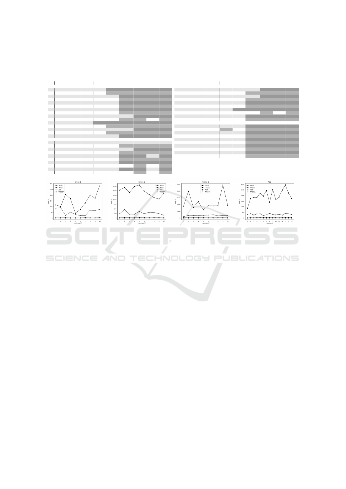
Table 1: Results for the instances introduced by (Ferdous and Rahman, 2017). Columns DD
W
contain the objective function
values obtained by using Decision diagrams with different restrictions on layer width. The remaining columns contain the
objective function values reported in (Blum et al., 2016) for the solution approaches considered in this paper. A cell is grey if
an approach considered in (Blum et al., 2016) obtains a better objective function value than all restricted DD
W
.
id DD
10
DD
100
DD
1000
greedy ACO TRESEA ILP
comp
heurILP CMSA
Real
1 92 88 88 93 87 86 78 85 78.9
2 160 160 157 160 155 153 139 150 140
3 120 117 116 119 116 113 104 112 104.7
4 164 162 161 171 164 156 144 158 143.7
5 169 169 168 172 171 166 150 161 152.9
6 149 146 144 153 145 143 128 139 127.6
7 138 136 134 135 140 131 121 132 122.7
8 136 131 129 133 130 128 116 123 118.4
9 144 141 143 149 146 142 131 139 130.7
10 148 147 144 151 148 143 131 144 131.7
11 125 125 126 124 124 120 110 122 111.9
12 141 141 142 143 137 138 126 136 127.5
13 177 175 172 180 180 172 156 171 158.6
14 151 151 152 150 147 146 134 147 134
15 155 153 153 157 160 152 139 148 141.7
Group 1
1 44 44 41 46 42 42 41 42 41
2 53 51 50 54 51 48 47 48 47
3 60 57 55 60 55 55 52 54 52
4 45 45 45 46 43 43 41 43 41
5 45 44 43 44 43 41 40 43 40
6 45 46 45 48 42 41 40 41 40
7 62 62 60 64 60 59 55 59 56
8 47 44 44 47 47 45 43 44 43
9 47 46 45 42 45 43 42 48 42
10 61 58 58 63 59 58 54 58 54
id DD
10
DD
100
DD
1000
greedy ACO TRESEA ILP
comp
heurILP CMSA
Group 2
1 116 112 109 118 113 111 98 108 101.2
2 114 116 115 121 118 114 106 111 104.6
3 115 107 110 114 111 107 97 105 97.1
4 118 115 112 116 115 110 102 111 102.5
5 138 134 129 132 132 127 116 125 117.8
6 106 107 105 107 105 102 93 101 95.4
7 101 99 99 106 98 95 88 96 89
8 116 117 113 122 118 114 104 116 105.2
9 123 117 116 123 119 113 104 112 104.9
10 103 100 99 102 101 97 89 94 89.8
Group 3
1 180 175 175 181 177 171 155 173 157.9
2 178 174 175 173 175 168 155 165 157.5
3 194 188 188 195 187 185 166 180 167.3
4 188 184 182 191 184 179 159 171 161.8
5 170 172 168 174 171 162 150 164 151.1
6 162 164 168 169 160 162 147 155 149.3
7 169 167 167 171 167 159 149 160 147.8
8 175 178 171 185 175 170 151 166 154.2
9 175 174 172 174 172 169 158 169 155.3
10 163 163 161 171 167 160 148 160 149
Figure 1: Runtime of the DD
W
experiments with comparison to ACO and TRESEA.
objective function value obtained for all instances of
the same configurations.
As we can see in Figure 1, the DD approach runs
faster than ACO and in most cases computes a bet-
ter MCSP objective function values, as can be seen in
Table 1. The ACO runs at least 30× slower on 93%
of instances. The runtime difference is over 2000 sec-
onds for 20% of instances.
As we can see in Tables 1 and 2, TRESEA and
the DD approach behave similarly. For smaller in-
stances of the MCSP, TRESEA outperforms the re-
stricted DD. However, for instances of the MCSP on
longer strings on alphabets |Σ| ∈ {12,20} the DD ap-
proach computes better objective function value on
the MCSP than the TRESEA approach. As we can see
in Figure 1 the DD even has a better runtime. TRE-
SEA is at least 6× slower for 93% of instances than
the DD approach.
The Greedy approach (Chrobak et al., 2004; He,
2007) is very similar to our approach of DD
1
. As we
can see in both Tables 1 and 2 the restricted DDs with
bigger layer width gives better bounds.
The main advantage of the DD is the runtime com-
pared with basic the ILP models. The runtime needed
to get objective function values from the ILP mod-
els grows fast with the instance size in comparison
with the DD. This can be seen in both tables 1 and 2.
The DD get worse bounds than ILP in case of enough
time. However, as the instances grow, the DD gets
better objective function values in a given time. The
DD approach is 50× faster for 50% of instances then
the CSMA approach.
5 CONCLUSION
In this work, we developed a DP formulation for the
MCSP. Based on this DP formulation we designed an
exact DD solution approach and a heuristic solution
approach using a restricted version of this DD. The
exact DD is not suitable for solving large instances of
the MCSP as the runtime grows exponentially. The
restricted DD scales much better and can be used to
heuristically solve the MCSP with much larger input.
We use the datasets from literature (Blum et al., 2016;
Ferdous and Rahman, 2017) to compare our DD ap-
proach with existing approaches such as Greedy ap-
proach (Chrobak et al., 2004; He, 2007), ACO (Fer-
dous and Rahman, 2017), TRESEA (Blum et al.,
2014) and various ILP based models (Blum et al.,
2015; Blum et al., 2016).
In our experiments we have shown our approach
is better than the Greedy approach and ACO both in
ICORES 2022 - 11th International Conference on Operations Research and Enterprise Systems
182

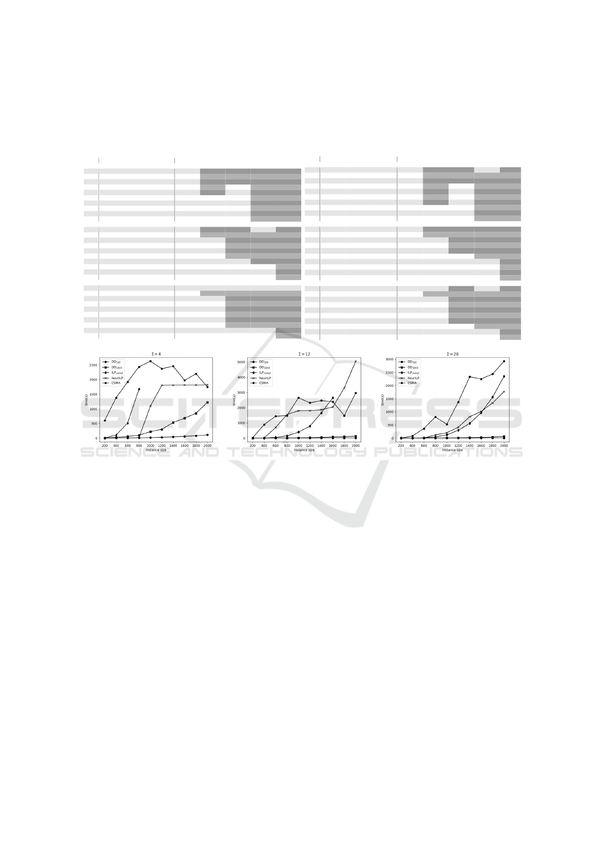
Table 2: Results for the instances introduced by (Blum et al., 2016), averaged by instances of the same configuration. Columns
DD
W
contain the objective function values obtained by using Decision diagrams with different restrictions on layer width.
The remaining columns contain the objective function values reported in (Blum et al., 2016) for the solution approaches
considered in this paper. A cell is grey if an approach considered in (Blum et al., 2016) obtains a better objective function
value than all restricted DD
W
.
linear
n DD
10
DD
100
DD
1000
greedy TRESEA ILP
comp
heurILP CMSA
Σ = 4
200 73.6 72 70.5 75 68.7 63.5 69 63.7
400 132.2 129.6 128.3 133.4 126.1 115.7 124.3 116.4
600 182.6 180.4 179 183.7 177.5 162.2 174.1 162.9
800 238.2 235.5 233.1 241.1 232.7 246.8 229.1 212.4
1000 285.7 284.5 284 287 280.4 n/a 277.2 256.9
1200 333.9 330.9 329 333.8 330.4 n/a 324.8 303.3
1400 383.8 382.3 378.9 385.5 378.9 n/a 373.1 351
1600 429.4 424.4 422.8 432.3 427.1 n/a 416.7 400.6
1800 476.4 473.6 471.1 477.4 474.2 n/a 464.4 445.4
2000 521.2 519.4 512.9 521.6 520.7 n/a 512.7 494
Σ = 12
200 124.5 123.3 122.2 127.3 122.1 119.2 123 119.2
400 227.5 225.8 224.1 228.9 223.5 208.9 215.7 209.4
600 320.8 318.1 317.9 322.2 318.7 291 296.2 293.8
800 412.8 409.3 405.3 411.4 408.1 368.7 373.9 373.2
1000 497 494.1 491.5 499.2 494.9 453.4 452 449.9
1200 586.2 581.2 578.5 586 585.6 536.6 542.4 531
1400 663.7 658.1 657.9 666 664.6 684.1 653.3 606.9
1600 751.7 749.3 744.1 754.4 754.6 773.5 749.7 694.8
1800 829.5 826.3 820.3 827.3 833 n/a 850.7 773.6
2000 913.1 909.1 904.6 913.5 916.2 n/a 939.6 849.6
Σ = 20
200 147.7 146.7 146.1 149.2 146.6 146.2 146.4 146.2
400 272.4 270.4 269.6 274.5 268.8 261.5 263.8 261.9
600 387.9 385.4 383 389.2 383.5 362.3 369.3 366.6
800 493 489.9 487.5 495.8 492.3 456.1 464.7 463.1
1000 600 595.7 594 600.6 597.5 547.1 562.5 555
1200 705.5 701.2 697.4 706.1 707.8 642.2 658.8 648.5
1400 800.5 796.2 793.4 801.1 804 737.9 745.7 737.7
1600 902.6 898.3 896.5 899.8 903.1 861.3 872.6 825.7
1800 997.2 992.6 988.7 996.8 1000.1 1012.9 994.4 917.6
2000 1095.8 1094.2 1086.4 1097.8 1102.6 1136 1120.7 1024.9
skewed
n DD
10
DD
100
DD
1000
greedy TRESEA ILP
comp
heurILP CMSA
Σ = 4
200 67.8 66.2 64.2 68.7 62.8 57.4 64.6 57.5
400 120.5 118.9 117.2 120.3 115 105.3 116.5 105.1
600 169.5 167.6 165.4 170.6 163.8 149.7 165.2 150.4
800 220 216.2 214.7 219.8 213.3 224 211.7 196.5
1000 265.8 265.8 263.2 268.6 261.7 n/a 260.1 240.2
1200 315.9 311.5 309.3 313.8 309 n/a 302.1 285
1400 362.3 357.4 354.3 358.7 352.2 n/a 346 327.6
1600 403.7 401.4 397.1 400.9 397.9 n/a 394.4 376
1800 444.1 438.4 438.5 440.6 442.1 n/a 431.7 417.7
2000 486.1 482.6 476.9 485 481.2 n/a 468.9 470.2
Σ = 12
200 115.5 114.3 114 117.9 112.7 108.5 112.7 108.6
400 214.1 210.8 210.3 216.1 208.5 193.4 197.6 194.3
600 305.1 304.3 300.4 304.8 301.7 274.5 277.9 277.2
800 388.8 385.4 381.9 389.3 385.4 347 348.8 351
1000 469.4 468.6 464 471.6 468.9 429.4 428.7 424.4
1200 550.5 545.7 544.1 551.1 549.9 559.4 535 500.1
1400 626.7 621.7 622.7 625.7 626.3 645.1 638.4 570
1600 704.1 699.7 694.5 705.6 706.4 n/a 715.1 643.8
1800 786.4 784.5 781.7 788.4 788.9 n/a 810.1 723.3
2000 859.2 854.3 848.8 857.8 858 n/a 879.9 797.3
Σ = 20
200 138.1 136.8 135.6 140.4 135.9 134.7 136.5 134.7
400 255 253 251.7 255.5 251.3 240.3 246.1 240.6
600 364.3 362.6 360.3 366.8 361.2 336.1 344.6 341.1
800 465.4 461.1 459.5 466.3 462.7 424.4 429.9 429.8
1000 569.2 565.4 561.8 567.6 566.6 514.7 525 520.9
1200 661.1 657.9 656 661.8 662.4 604.2 608.2 605.7
1400 756.9 755 751.7 762.3 760.7 694.4 696.1 693.2
1600 850 847.1 844.6 851.2 855.2 863.3 838.9 780.4
1800 946.4 941.2 937.5 948.7 948.8 969.8 964.7 870.2
2000 1033.9 1029.1 1025.6 1034.3 1037.7 1061.6 1066.6 967.1
Figure 2: Runtime of DD
W
experiments with comparison to the ILP models on instance-set linear with |Σ| = 4,12, 20. The
line for ILP
compl
ends sooner as it did not return any feasible solution after an hour for missing lines.
the obtained objective function values and the run-
time. Moreover, it obtains better objective function
values for the MCSP with bigger alphabets and longer
strings than TRESEA, ILP
compl
and heruILP in a
given time. The CSMA obtains better results than our
approach, however, it is much slower.
A potential next research step could be improving
the heuristic for variable ordering and node ordering
of the restricted DD together with a better heuristic for
the layer width restriction. Another avenue for further
research could be to hybridize the DD model with the
ILP model. The DD model runs fast and its simplicity
allows to include any heuristic in any node to serve as
the criterion to delete such node with its descendants
and get the restricted DD computing better objective
function values. We hope that it could compete with
the CSMA approach.
Future Work. Here we present some additional ideas
in which way future research could be directed.
1. Current implementation builds the DD breadth-
first. We could change the order of processed
nodes by using the priority queue instead process-
ing whole layer at once. The node order can be
for example
• combination of the value of r-n
i
path and the
number of yet uncovered symbols (A
∗
ap-
proach),
• bounds by more restricted or relaxed DD or by
ILP on subproblem defined by node n
i
. The de-
cision to use either DD or ILP for bounds can
be made by Machine learning methods as Gon-
zales et al. used for a Maximum independent
set problem (Gonz
´
alez et al., 2020).
2. Change the strategy of choosing node deleted dur-
ing the restriction step. Our implementation uses
a linear approach with the newly created layer’s
size, significantly speeding up the algorithm. We
can change the speed for some more complex val-
uation of nodes.
3. In our work, we only implemented a restricted DD
for the MCSP, which gives us the upper bound
On Solving the Minimum Common String Partition Problem by Decision Diagrams
183

of the optimal objective function value. For the
lower bound, we can use a relaxed DD (Bergman
et al., 2016). The main advantage of such an ap-
proach would be that the relaxed DD can be incre-
mentally refined to get better solutions. We have
already tried a few relaxations. However, we ob-
tained a very weak lower bound on the MCSP. We
are interested in a suitable method for relaxation
yielding better lower bounds in a reasonable time.
ACKNOWLEDGEMENTS
This work was supported by the JKU Business
School.
REFERENCES
Bergman, D., Cire, A. A., Hoeve, W.-J. v., and Hooker, J.
(2016). Decision Diagrams for Optimization. Ar-
tificial Intelligence: Foundations, Theory, and Algo-
rithms. Springer International Publishing.
Blum, C. (2020). Minimum common string partition: on
solving large-scale problem instances. International
Transactions in Operational Research, 27(1):91–111.
Blum, C., Lozano, J. A., and Davidson, P. (2015). Mathe-
matical programming strategies for solving the min-
imum common string partition problem. European
Journal of Operational Research, 242(3):769–777.
Blum, C., Lozano, J. A., and Pinacho Davidson, P. (2014).
Iterative Probabilistic Tree Search for the Minimum
Common String Partition Problem. In Hybrid Meta-
heuristics, Lecture Notes in Computer Science, pages
145–154, Cham. Springer International Publishing.
Blum, C., Pinacho, P., L
´
opez-Ib
´
a
˜
nez, M., and Lozano, J. A.
(2016). Construct, Merge, Solve & Adapt A new gen-
eral algorithm for combinatorial optimization. Com-
puters & Operations Research, 68:75–88.
Blum, C. and Raidl, G. R. (2016). Computational Per-
formance Evaluation of Two Integer Linear Program-
ming Models for the Minimum Common String Par-
tition Problem. Optimization Letters, 10(1):189–205.
arXiv: 1501.02388.
Chen, X., Zheng, J., Fu, Z., Nan, P., Zhong, Y., Lonardi,
S., and Jiang, T. (2005). Assignment of orthologous
genes via genome rearrangement. IEEE/ACM trans-
actions on computational biology and bioinformatics,
2(4):302–315.
Chrobak, M., Kolman, P., and Sgall, J. (2004). The Greedy
Algorithm for the Minimum Common String Parti-
tion Problem. In Approximation, Randomization, and
Combinatorial Optimization. Algorithms and Tech-
niques, Lecture Notes in Computer Science, pages
84–95, Berlin, Heidelberg. Springer.
Ferdous, S. M. and Rahman, M. S. (2017). Solving the
Minimum Common String Partition Problem with the
Help of Ants. Mathematics in Computer Science,
11(2):233–249.
Goldstein, A., Kolman, P., and Zheng, J. (2005). Min-
imum Common String Partition Problem: Hardness
and Approximations. In Algorithms and Computation,
Lecture Notes in Computer Science, pages 484–495,
Berlin, Heidelberg. Springer.
Gonz
´
alez, J. E., Cire, A. A., Lodi, A., and Rousseau, L.-M.
(2020). Integrated integer programming and decision
diagram search tree with an application to the maxi-
mum independent set problem. Constraints, 25(1):23–
46.
Gusfield, D. (1997). Algorithms on Strings, Trees, and Se-
quences: Computer Science and Computational Biol-
ogy. Cambridge University Press, Cambridge.
He, D. (2007). A Novel Greedy Algorithm for the Min-
imum Common String Partition Problem. In Bioin-
formatics Research and Applications, pages 441–452,
Berlin, Heidelberg. Springer.
Horn, M., Djukanovic, M., Blum, C., and Raidl, G. R.
(2020). On the Use of Decision Diagrams for Find-
ing Repetition-Free Longest Common Subsequences.
In Optimization and Applications, Lecture Notes in
Computer Science, pages 134–149. Springer Interna-
tional Publishing, Cham.
Hosseininasab, A., Hoeve, W.-J., and Cire, A. (2019).
Constraint-Based Sequential Pattern Mining with De-
cision Diagrams. Proceedings of the AAAI Conference
on Artificial Intelligence, 33:1495–1502.
Hosseininasab, A. and van Hoeve, W.-J. (2021). Exact
Multiple Sequence Alignment by Synchronized De-
cision Diagrams. INFORMS Journal on Computing,
33(2):721–738. Publisher: INFORMS.
Hsu, W. J. and Du, M. W. (1984). Computing a longest
common subsequence for a set of strings. BIT Numer-
ical Mathematics, 24(1):45–59.
Meneses, C. N., Oliveira, C. A. S., and Pardalos, P. M.
(2005). Optimization techniques for string selection
and comparison problems in genomics. IEEE Engi-
neering in Medicine and Biology Magazine, 24(3):81–
87.
Mousavi, S. R., Babaie, M., and Montazerian, M. (2012).
An improved heuristic for the far from most strings
problem. Journal of Heuristics, 18(2):239–262.
Smith, T. F. and Waterman, M. S. (1981). Identification of
common molecular subsequences. Journal of Molec-
ular Biology, 147(1):195–197.
Tjandraatmadja, C. (2018). Decision Diagram Relaxations
for Integer Programming. Dissertation, Decision Dia-
gram Relaxations for Integer Programming.
van Hoeve, W.-J. (2020). Graph Coloring Lower Bounds
from Decision Diagrams. In Integer Programming
and Combinatorial Optimization, pages 405–418,
Cham. Springer International Publishing.
ICORES 2022 - 11th International Conference on Operations Research and Enterprise Systems
184