Prognostic-based Maintenance Optimization in Complex Systems with

Resource Limitation Constraints

Junkai He

1 a

, Miguel F. Anjos

2 b

, Makhlouf Hadji

1 c

and Selma Khebbache

1 d

Technological Research Institute SystemX, 8 Avenue de la Vauve, 91120 Palaiseau, France

School of Mathematics, University of Edinburgh, Peter Guthrie Tait Road, Edinburgh EH9 3FD, Scotland, U.K.

Keywords:

Predictive Maintenance, Optimization, Complex System, Prognostic Information, Remaining Useful Life,

Resource Limitation.

Abstract:

This paper is concerned with prognostic information for maintenance optimization in complex systems. At

each stage of such a system, we consider redundant components used as backup to guarantee the system’s

availability. The Remaining Useful Life (RUL/prognostic information) of components is used to evaluate

each component’s redundancy. We address RUL-based maintenance optimization under resource limitation

to ensure the availability of the system such that production demands can be satisﬁed in a given maintenance

planning horizon. We propose a mixed-integer linear programming approach to minimize the overall cost. Our

numerical results on test instances show the efﬁciency of the proposed approach to attain optimal solutions.

1 INTRODUCTION

Industrial systems generally degrade due to different

factors. This degradation may eventually cause seri-

ous economic problems for companies. Maintenance

is a widely recognized essential element in asset man-

agement to reduce the speed of degradation (De Jonge

and Scarf, 2020). However, traditional maintenance

decisions for single-component systems are not suit-

able for contemporary complex systems. Complex

systems are systems that are difﬁcult to categorize

as series, parallel, or k/n networks. They commonly

consist of multiple components with various interac-

tions (Zhu et al., 2021). Industrial and academic re-

searchers have thus been focusing on proposing ef-

fective maintenance optimization strategies for such

complex systems.

In industrial applications, maintenance is mainly

classiﬁed as Corrective Maintenance (CM) and Pre-

ventive Maintenance (PM). CM is carried out when

a component has broken down, while PM happens in

advance to reduce the degradation speed and avoid a

sudden failure. In addition, these two maintenance

types are often considered under resource constraints

https://orcid.org/0000-0003-0918-876X

https://orcid.org/0000-0002-8258-9116

https://orcid.org/0000-0003-1048-753X

https://orcid.org/0000-0001-5248-2548

that represent the limited number of available techni-

cians, repairmen, apparatus, etc. If and only if enough

resource is provided, the maintenance can be con-

ducted and accomplished.

To make decisions about maintenance policies, an

interesting approach consists of soliciting the prog-

nostic information of components, such as the Re-

maining Useful Life (RUL) (Camci et al., 2019). The

deﬁnition of component’s RUL is the currently re-

maining time of operation before it fails. The focus

of our work is on using the obtained component-level

RUL information to plan PM optimization in order to

achieve system-level availability in complex systems.

We consider generic complex systems with a se-

ries of stages and each stage contains multiple redun-

dant components (see Figure 1). The same type of

structure has been considered in multi-process indus-

tries, such as gas production (Ye et al., 2019; Xenos

et al., 2016). The overall aim consists in coordinating

the operations in different stages and provides global

maintenance decisions such that the system can oper-

ate continuously during the planning horizon to sat-

isfy client demands. This approach can be seen as an

integration of maintenance and production.

In summary, we address a RUL-Based Mainte-

nance Optimization (RBMO) problem in complex

systems with resource limitation constraints (RBMO-

RL). The objective is to minimize the total cost over

a planning optimization horizon, including mainte-

He, J., Anjos, M., Hadji, M. and Khebbache, S.

Prognostic-based Maintenance Optimization in Complex Systems with Resource Limitation Constraints.

DOI: 10.5220/0010829100003117

In Proceedings of the 11th International Conference on Operations Research and Enterprise Systems (ICORES 2022), pages 169-176

ISBN: 978-989-758-548-7; ISSN: 2184-4372

169

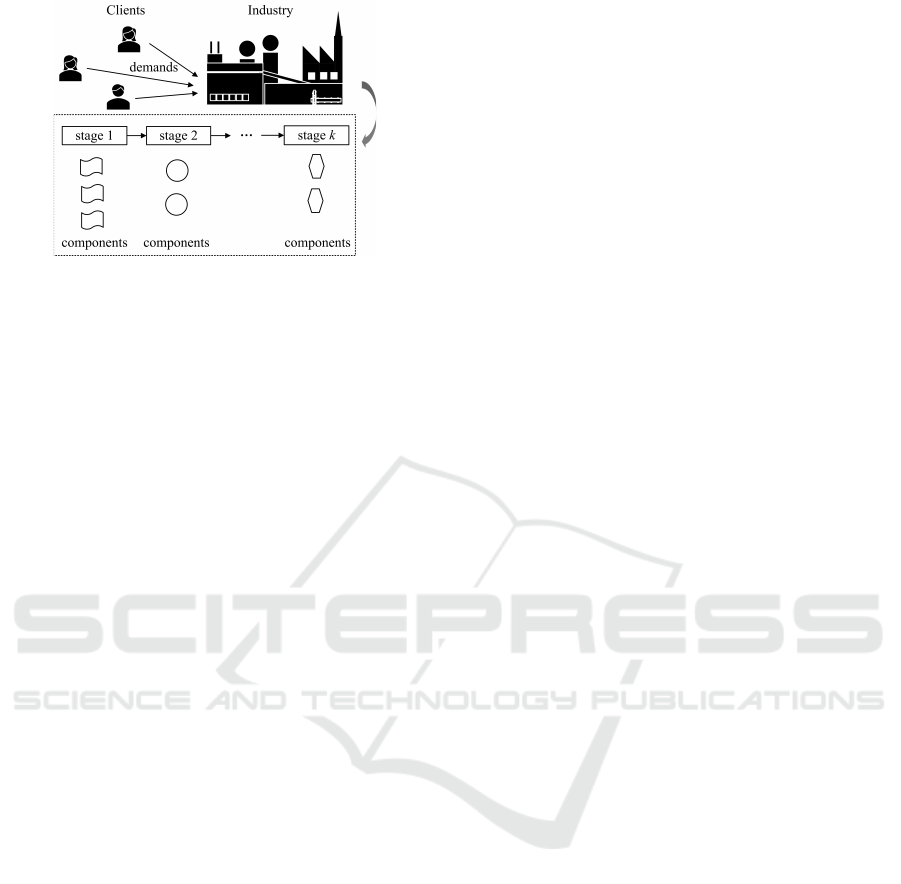
Figure 1: Architecture of the studied complex systems.

nance cost, system-failure cost, inventory expense,

and a penalty for non-met production. The contribu-

tions in our work are as follows:

• A novel RBMO-RL problem to minimize the total

cost in complex systems.

• A Mixed-Integer Linear Programming (MILP)

formulation of this problem.

The remaining of this paper is organized as fol-

lows. In Section 2, we review related literature to

highlight and position our contributions. In Section 3,

we mathematically formulate the RBMO and RBMO-

RL problems and provide MILP models. Numerical

tests are conducted and the results are reported and

analyzed in Section 4. Section 5 is dedicated to the

conclusion and future work.

2 LITERATURE REVIEW

2.1 Maintenance in Complex Systems

We review the main contributions in the maintenance

literature concerned with RUL usage, system avail-

ability, and integrated problems.

RUL is an essential index that reﬂects the status of

a component. In general, it can be either obtained by

deﬁning the time length from the current time to the

end-of-life. Or more frequently, it is deﬁned as the

time left before the health condition reaches a warn-

ing threshold (Si et al., 2011). More than 270 pa-

pers have studied RUL prediction (Lei et al., 2018).

We focus on RUL usage in our work and distinguish

three branches in the literature. (i) RUL-based in-

spection: Do et al. (2015) used RUL information for

deciding the time point for the next coming inspec-

tion. (ii) RUL-based maintenance strategies: Chen

et al. (2019) proposed different maintenance actions

via combinations of degradation and RUL. (iii) RUL-

based constraints: Camci et al. (2019) used prognos-

tic information to formulate probability constraints

related to the failure rate of a component.

For describing system-level availability by com-

ponent condition, Wu and Castro (2020) proposed a

linear combination of the degradation processes of

several components. If this value exceeded a given

threshold, PM was performed. Lei and Sandborn

(2018) proposed a prognostic health analysis to pre-

dict the RUL of wind turbines. The authors assumed

that turbines were dependent and system availability

relied on the minimum RUL among them. Dong et

al. (2020) assumed that normal-distributed shocks oc-

curred independently and described system reliability

by conditioning on the numbers of arrived shocks.

Integrated problems combine maintenance in

complex systems with other scopes to make global

decisions. One of the mainstream approaches is to si-

multaneously take maintenance and resource into ac-

count, such as spare part ordering. Camci (2009) pro-

posed CM and spare part inventory strategies using

the given prognostic information to minimize the fail-

ure risk. A genetic algorithm was proposed to solve

the problem and computational results were com-

pared with the ones via PM strategy. Numerous pa-

pers have considered spare part ordering, see the in-

vited review (De Jonge and Scarf, 2020). The integra-

tion of maintenance and production is also an impor-

tant branch because maintenance activities eventually

impact production. Bahria et al. (2019) developed

an integrated approach to control production, main-

tenance, and quality for manufacturing. Appropri-

ate thresholds for conducting maintenance were dis-

cussed to guarantee the robustness of the system.

From the literature, we observe a lack of RUL us-

age and mathematical modeling via RUL-based con-

straints. Moreover, the inﬂuence of individual RUL

information on complex systems is seldom discussed.

Hence, and to the best of our knowledge, the inte-

grated optimization of maintenance and production

in series-structured systems with backup components

and resource limitation has not been studied. In our

work, we address maintenance optimization for com-

plex systems considering standby components and re-

source limitation. The optimization aims to guaran-

tee the continuous operation of the system. This is

achieved by integrating component-level RUL infor-

mation in the formulation.

2.2 Maintenance Optimization Methods

Many solution methods based on optimization for

maintenance problems in complex systems have been

proposed. In the following, we discuss some of the

related and recent references and clearly situate our

contribution compared to these approaches.

ICORES 2022 - 11th International Conference on Operations Research and Enterprise Systems

170

In the mentioned Camci (2009) and Xiao et al.

(2016), genetic algorithms were proposed to solve the

problems. Rivera-G

omez et al. (2020) presented a

continuous production system with quality deteriora-

tion. The objective was to reduce the occurred cost

with a quality constraint. A non-linear programming

model was formulated for the problem. Zhou et al.

(2019) proposed an optimal PM policy with the pur-

pose to get operational parameters for a production

line. A non-linear model and a heuristic were de-

signed to minimize the cost and guarantee the oper-

ating speed. Compared to the widely used non-linear

formulation and (meta-) heuristics, linear formulation

for maintenance optimization is very limited. In this

research, we formulate MILP models for the consid-

ered RBMO and RBMO-RL problems, with the pur-

pose to provide optimal maintenance decisions.

3 PROBLEM DESCRIPTION AND

FORMULATION

3.1 RBMO Problem Description

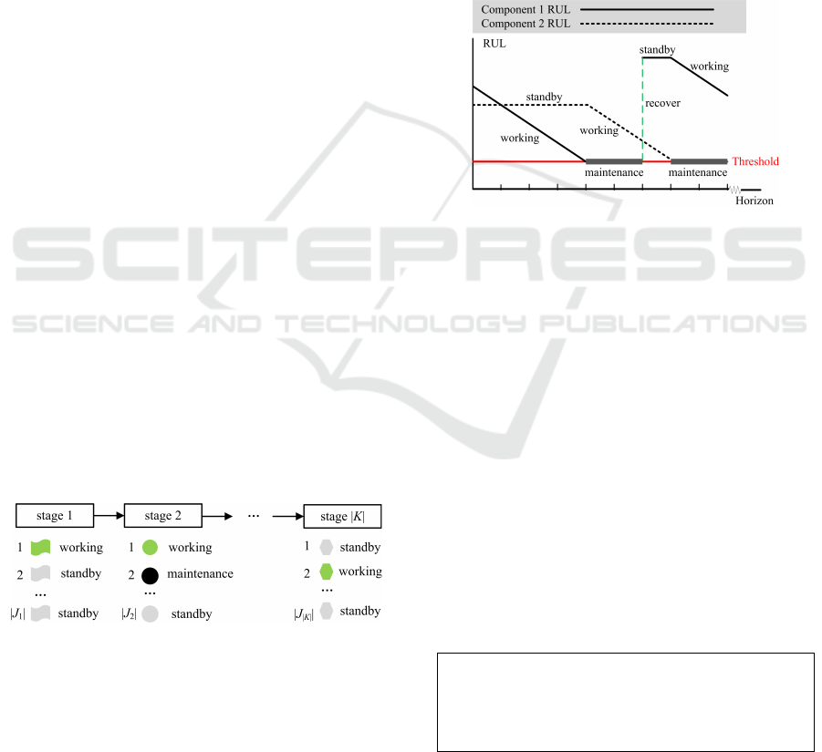
The architecture of the considered complex systems

in Figure 2 contains |K| processing stages where K

denotes the stage set. Stage k (∈ K) is conﬁgured with

| components where J

represents the component

set in stage k. Each component may have three states:

working (in green), standby (in grey), and mainte-

nance (in black), respectively. We assume that each

component is repairable, and that maintaining it does

not affect the operation of a stage if there exist any

available standby component. The planning horizon

contains |T | periods (weeks), where T is the period

set. The purpose is to satisfy the demands of |I| clients

during this horizon, where I is the client set.

Figure 2: Schematic diagram of the complex system.

We now describe the three main sets of constraints

in our model in the following.

Evolution of RUL over time. The model keeps

track of the RUL of components over the optimiza-

tion horizon. It is assumed that the prognostic RUL

of component j in stage k follows a linear function

k, j

− a

k, j

· t, where a

k, j

and b

k, j

respectively denote

the coefﬁcient and constant. Note that RUL can be al-

ternatively described using values, quantiles, or prob-

abilities. We choose the ﬁrst option in this research,

and leave the other ones for future work. As illus-

trated in Figure 3, for component j in stage k, if it is

operating during a period, its RUL decreases in value

by a

k, j

. If it is standby, its RUL will not change. If it

is under maintenance, its RUL will stay at the thresh-

old γ

until maintenance is carried out. Note that any

component reaching the corresponding threshold can

no longer operate and needs to be maintained. After

maintenance, its RUL is restored to b

k, j

. The initial

RUL of each component is given as o

k, j

. We assume

that threshold γ

is provided by experts. Hence, opti-

mizing γ

is outside the scope of this paper.

Figure 3: Evolution of RUL.

System Availability. The operation of a stage re-

quires that at least one component (at the same stage)

is working. If not, it eventually results in the unavail-

ability of the system because it operates if and only if

all stages are working.

Production Integration. The system has a produc-

tion of qua

in period t to satisfy demands d

. How-

ever, its production capacity for each period is lim-

ited by Q. If the system cannot work during a period,

there is no production and it may cause some produc-

tion loss. To avoid demand unmet, we allow some

possible stocks in preparation (if needed) to serve for

subsequent client demands.

3.2 RBMO Formulation

Before introducing our mathematical model for the

RBMO problem, and for sake of clarity, we summa-

rize the notations that will be used in our formulation.

Problem sets

- I: set of clients;

- K: set of stages in the system;

- J

: set of components in stage k;

- T : set of periods;

Prognostic-based Maintenance Optimization in Complex Systems with Resource Limitation Constraints

171

Parameters:

- cap: production capacity of the system each period;

- a

k, j

: coefﬁcient in the RUL function of component j

in stage k;

- b

k, j

: constant in the RUL function of component j in

stage k; then the RUL function can be established by

k, j

− a

k, j

·t;

- o

k, j

: original RUL of component j in stage k;

- γ

: RUL threshold of components in stage k;

- p

: maintenance duration of components in stage k;

- d

: demand of client i in period t;

- c

: unit maintenance cost;

- c

: unit failure cost;

- c

Inv

: unit inventory cost;

- c

Loss

: unit production-loss cost.

Decision variables:

- x

k, j

: binary variable, equals to 1 if component j in

stage k needs to be maintained in period t, 0 otherwise;

- y

k, j

: binary variable, equals to 1 if component j in

stage k is working in period t, 0 otherwise;

- R

k, j

: RUL of component j in stage k in period t;

- ST

: binary variable, equals to 1 if stage k is working

in period t, 0 otherwise;

- SY

: binary variable, equals to 1 if the system is work-

ing in period t, 0 otherwise;

- qua

: production quantity in period t;

- inv

: inventory in period t. Note that there is no in-

ventory at the beginning of the horizon;

- z

: binary variable, equals to 1 if the inventory is pos-

itive in period t, 0 otherwise.

The MILP model for the RBMO problem is for-

mulated and noted by (M1). We consider the objec-

tive function (1) as the sum of four terms:

• C

denotes the total maintenance cost that is cal-

culated by unit maintenance cost times the num-

ber of maintenance activities.

• C

denotes the total failure cost that is computed

by unit failure cost times the number of failures.

• C

Inv

denotes the total inventory cost that is com-

puted by unit inventory cost times the amount of

inventory (if any).

• C

Loss

denotes the total production-loss cost that is

computed by unit production-loss cost times nega-

tive inventory. Here negative inventory represents

the quantity of unsatisﬁed demands.

(M1) : minC

Inv

Loss

(1)

= c

∑

k∈K

∑

j∈J

∑

t∈T

k, j

= c

∑

t∈T

(1 − SY

)

Inv

= c

Inv

∑

t∈T

· inv

Loss

= c

Loss

∑

t∈T

(1 − z

) · inv

Note that the non-linear term z

· inv

can be lin-

earized by introducing an auxiliary variable µ

= z

inv

with two additional constraints inv

≤ µ

+ M ·

(1 − z

) and 0 ≤ µ

+ M · z

. However, we chose to

let CPLEX handle these terms automatically (IBM).

The optimization of formula (1) is under the fol-

lowing sets of constraints:

Evolution of RUL Constraints. This constraint

group is formulated to track the RUL of components.

To be more speciﬁc, a maintenance is required when

the RUL of a component is no bigger than the cor-

responding threshold, which is guaranteed by con-

straints (2) and (3). If a component is under mainte-

nance, its unavailable time respects the maintenance

duration, which is calculated by constraints (4). Con-

straints (5) restricts that only one component can be

working in each stage if there is a need. Evolution of

RUL contains three cases: (i) if a component is main-

tained, its RUL will be restored to a given value, that

is, R

t+1

k, j

= b

k, j

if x

k, j

= 1. Please refer to constraints

(6) to (7); (ii) If a component is being used in a period,

its RUL will decrease respecting the given RUL func-

tion, that is, R

t+1

k, j

= R

k, j

−a

k, j

if x

k, j

= 0 and y

k, j

= 1,

which is calculated by constraints (8) to (9); (iii) The

RUL of standby components will not change, that is,

t+1

k, j

= R

k, j

if x

k, j

= 0 and y

k, j

= 0, which is estab-

lished by (10) to (11).

k, j

> γ

− M · x

k, j

, ∀k ∈ K, j ∈ J

,t ∈ T (2)

k, j

≤ γ

+ M · (1 − x

k, j

), ∀k ∈ K, j ∈ J

,t ∈ T (3)

∑

∈[t,t+p

−1]

k, j

≤ 1 − x

k, j

∀k ∈ K, j ∈ J

,t ∈ [1, |T | − p

+ 1] (4)

∑

j∈J

k, j

≤ 1, ∀k ∈ K, t ∈ T (5)

t+1

k, j

≥ b

k, j

− M · (1 − x

k, j

∀k ∈ K, j ∈ J

,t ∈ [1, |T | − 1] (6)

t+1

k, j

≤ b

k, j

+ M · (1 − x

k, j

∀k ∈ K, j ∈ J

,t ∈ [1, |T | − 1] (7)

t+1

k, j

≥ R

k, j

− a

k, j

− M · (1 − y

k, j

∀k ∈ K, j ∈ J

,t ∈ [1, |T | − 1] (8)

t+1

k, j

≤ R

k, j

− a

k, j

+ M · (1 − y

k, j

∀k ∈ K, j ∈ J

,t ∈ [1, |T | − 1] (9)

t+1

k, j

≥ R

k, j

− M · (x

k, j

+ y

k, j

∀k ∈ K, j ∈ J

,t ∈ [1, |T | − 1] (10)

t+1

k, j

≤ R

k, j

+ M · (x

k, j

+ y

k, j

∀k ∈ K, j ∈ J

,t ∈ [1, |T | − 1] (11)

ICORES 2022 - 11th International Conference on Operations Research and Enterprise Systems

172

System Availability Constraints. This set of valid

inequalities describes stage availability and further

system availability for each period via the compo-

nents’ RUL information. The premise that a stage

operates normally is that at least one component in

the stage is working, i.e., ∃y

k, j

= 1. To this end, the

availability of a stage can be described by constraints

(12). For system availability, it strictly requires that

all the stages are available, i.e., ∀ST

= 1, which is

expressed by constraints (13) and (14).

≤

∑

j∈J

k, j

, ∀k ∈ K,t ∈ T

|K|

∑

k∈K

≤ SY

∑

k∈K

(1 − ST

), ∀t ∈ T

≥ SY

, ∀k ∈ K,t ∈ T

(12)

(13)

(14)

Production Integration Constraints. These con-

straints describe how system availability impacts pro-

duction and inventory. Constraints (15) provide the

upper bound of production quantity in each period

respecting system production capacity, while con-

straints (16) give the lower bound because a system

cannot produce if any one of the stages is not active.

The inventory is calculated by the sum of production

quantity and the inventory in the last period minuses

the currently total demands (constraints (17)). Note

that the inventory can be negative if the maintenance

leads to a non-working state for the system or produc-

tion capacity is surpassed. Then, constraints (18) and

(19) record that the on-hand inventory is non-negative

and negative, respectively, meaning that the inventory

is enough or not for satisfying client demands.

qua

≤ cap · ST

, ∀k ∈ K, t ∈ T (15)

qua

≥

∑

j∈J

k, j

, ∀k ∈ K, t ∈ T (16)

inv

= qua

+ inv

t−1

−

∑

i∈I

, ∀t ∈ T (17)

inv

≥ −M · (1 − z

), ∀t ∈ T (18)

inv

≤ M · z

, ∀t ∈ T (19)

Note that the initial RUL of a component is equal

to o

k, j

and there is no inventory at the beginning of

the planning horizon. The ranges of the decision vari-

ables are detailed as follows:

k, j

, y

k, j

, ST

, SY

, z

∈ {0, 1}, ∀k ∈ K, j ∈ J

,t ∈ T

k, j

, inv

, qua

∈ Z, ∀k ∈ K, j ∈ J

,t ∈ T

(20)

(21)

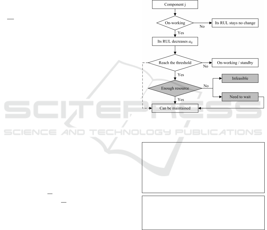
3.3 RBMO-RL Formulation

In this part, we assess the impact of resource limi-

tation constraints on maintenance optimization. As

shown in Figure 4, the main difference (grey icons)

between RBMO and RBMO-RL problems is whether

we have enough resources to do maintenance. If too

many components reach a warning condition at the

same time but resources are not enough, some of them

must wait for the maintenance. This waiting time can

be shortened or even be 0 by arranging component re-

dundancy. On the other hand, the RBMO-RL problem

can be infeasible if we cannot ﬁnd available resources

during the optimization horizon.

Figure 4: Impact of resource limitation.

We now proceed to formulate the resource limita-

tion constraints mathematically.

New parameters:

- n

: the number of resources required to maintain a

component in stage k;

- N

: the number of resources available in period t;

- e

: binary parameter, equals to 1 if the components

in stage k can start to be maintained in period t, 0 oth-

erwise. If N

≥ n

establishes for t

∈ [t + p

− 1], a

maintenance can be started in period t.

New decision variables:

- s

k, j

: binary variable, equals to 1 if component j in

stage k is started to be maintained in period t;

- o

k, j

: binary variable, equals to 1 if component j in

stage k is being maintained in period t.

k, j

≤

∑

∈[t,|T |]

k, j

, ∀k ∈ K, j ∈ J

,t ∈ T (22)

k, j

≤ e

, ∀k ∈ K, j ∈ J

,t ∈ T (23)

k, j

≤ o

k, j

(24)

∀k ∈ K, j ∈ J

,t ∈ [1, |T | − p

+ 1],t

∈ [t, t + p

− 1]

k, j

≤ 2 − x

k, j

− s

k, j

Prognostic-based Maintenance Optimization in Complex Systems with Resource Limitation Constraints

173

∀k ∈ K, j ∈ J

,t ∈ T, t

∈ [t, |T |],t1 ∈ [t, t

] (25)

k, j

≤ 1 − o

k, j

, ∀k ∈ K, j ∈ J

,t ∈ T (26)

∑

k∈K

∑

j∈J

· o

k, j

≤ N

, ∀t ∈ T (27)

k, j

, o

k, j

∈ {0, 1}, ∀k ∈ K, j ∈ J

,t ∈ T (28)

For resource limitation constraints, a maintenance

should start no earlier than the time when the RUL

of a component reaches the threshold, and it must

respect resource limitation, which are guaranteed by

constraints (22) and (23), respectively. Constraints

(25) provide the length of resource occupation dur-

ing maintenance. Once the RUL of a component

reaches the threshold, it cannot be used until the main-

tenance is ﬁnished. To be speciﬁc, constraints (25)

denote its unavailability during the wait while con-

straints (26) denote its unavailability during the main-

tenance. The resource limitation is veriﬁed by con-

straints (27), meaning that the total number of re-

sources for maintenance occupation must not exceed

the currently available resources. Finally, constraints

(28) provide the ranges of new variables.

We add a new term in the objective function re-

garding the earlier start time for maintenance. The

model for the RBMO-RL problem is established be-

low and noted by (M2).

(M2) : min C

Inv

Loss

∑

k∈K

∑

j∈J

∑

t∈T

t · s

k, j

subject to : (2) − (3), (5) − (20), (22) − (28)

4 COMPUTATIONAL RESULTS

In this section, computational tests are conducted to

compare the performance of the two provided mathe-

matical models. All the tests are conducted on a com-

puter with Core I7 and 8GB RAM system. The MILP

models are solved using CPLEX 12.8 in Python 3.7.8.

4.1 Test Instances

To illustrate the differences between the two mod-

els, we set up several instances with different sizes.

We describe the size of each instance as (|I|, |K|, |T |),

where these quantities are the number of clients,

stages, and periods, respectively. The tested sizes

include S1(5,5,6), S2(5,5,12), S3(5,10,12). In each

stage, the number of components |J

| is randomly

generated from the range [1, 8]. Note that Ye et al.

(2019) looks at the design of systems with the same

structure but considers instances with only up to |K| =

4 and |J

| = 3. (The number of clients and the number

of periods are not considered in this design problem.)

For each size, we have solved 10 independently

generated instances using both models (M1) and

(M2). The computational results are collected in Ta-

bles 1, 2, and 3, respectively. In these tables, the ﬁrst

column denotes the instance index in different sizes,

for example, ‘S1-1’ is the ﬁrst instance within size S1.

The columns labeled (M1) and (M2) report respec-

tively the results obtained by models (M1) and (M2),

including their optimal objective values (Obj), com-

puting times in seconds (T(s)), and Number of Main-

tenances (NoM). Besides, ’-’ denotes infeasibility of

model M2 for solving corresponding instances.

Table 1: Experimental results for size S1(5, 5, 6).

(M1) (M2)

ID Obj T(s) NoM Obj T(s) NoM

S1-1 102 0.3 0 102 0.3 0

S1-2 62 0.3 1 64 0.3 1

S1-3 46 0.4 0 46 0.4 0

S1-4 78 0.3 0 78 0.3 0

S1-5 143 0.3 0 143 0.3 0

S1-6 255 0.3 3 321 0.8 4

S1-7 103 0.3 1 108 0.3 1

S1-8 74 0.2 0 74 0.2 0

S1-9 493 0.3 1 497 0.4 1

S1-10 414 0.3 0 414 0.3 0

Table 2: Experimental results for size S2(5, 5, 12).

(M1) (M2)

ID Obj T(s) NoM Obj T(s) NoM

S2-1 641 14.9 3 655 49.5 3

S2-2 158 0.9 0 158 1.8 0

S2-3 490 1.4 1 3694 186 1

S2-4 285 2.7 2 358 6.6 3

S2-5 625 0.7 1 630 6.2 1

S2-6 470 2.8 1 473 3.9 1

S2-7 238 0.9 2 248 1.7 2

S2-8 760 2.8 1 765 1.9 1

S2-9 1173 4.4 3 - - -

S2-10 493 27.8 3 507 422 3

4.2 Analysis of Results

From the tables, we have the following observations.

(i) The optimal values obtained by model (M2) are

no smaller than the ones by model (M1). This

is due to two factors, namely the additional term

in the objective function and the additional con-

straints (see also (iv) below).

(ii) The computing time of model (M2) is generally

greater than that of model (M1). This makes

sense since the RBMO-RL problem is more com-

plicated than the RBMO problem.

ICORES 2022 - 11th International Conference on Operations Research and Enterprise Systems

174

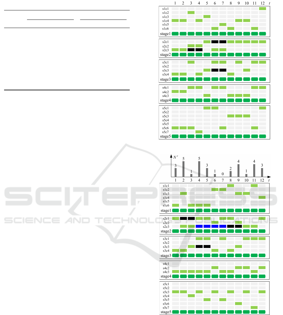
Table 3: Experimental results for size S3(5, 10, 12).

(M1) (M2)

ID Obj T(s) NoM Obj T(s) NoM

S3-1 408 162 6 ifsb - -

S3-2 352 4.9 2 367 11.0 2

S3-3 621 6.0 2 629 45.7 2

S3-4 954 5.4 1 957 7.9 1

S3-5 1322 5.2 4 1340 254 4

S3-6 2355 34.9 6 - - -

S3-7 966 2.1 1 977 8.1 1

S3-8 5675 5.7 1 5685 6.4 1

S3-9 367 5.6 1 370 9.4 1

S3-10 1146 5.3 2 1454 18.4 2

(iii) For the instances with ‘NoM = 0’, the objective

values obtained by the two models are the same.

The reason is that resource limitation is trivial if

there is no maintenance in the planning horizon.

(iv) The NoM obtained by model (M2) may be more

than that of model (M1). The reason is that, in

(M2), the waiting time for maintaining a com-

ponent is a part of unavailable time. Hence, an-

other component needs to operate to avoid system

breakdown, which may bring new maintenance.

However, model (M1) never has this trouble since

maintenance can be done once it occurs.

(v) Model (M1) always has feasible solutions because

maintenance can be done as soon as it is necessary

without needing to account for resource availabil-

ity. However, model (M2) may generate infeasi-

ble solutions if available resources cannot satisfy

maintenance needs in the planning horizon.

To sum up, considering resource limitations in

RBMO-RL (model (M2)) makes it more detailed than

RBMO (model (M1)) and changes the optimal main-

tenance plan. However, model (M2) is more realistic

because maintenance is usually done subject to avail-

able staff, equipment, etc.

4.3 Maintenance Decisions Comparison

In this part, we use an instance to distinguish main-

tenance decisions for the considered RBMO and

RBMO-RL problems. As shown in Figures 5 and 6,

the planning horizon contains 12 periods (horizontal

labels). The system consists of 5 stages and the ded-

icated number of components in each stage is given.

For example, ’s1c6’ represents component 6 in stage

1. For component’s states, the grey, green, blue, and

black rectangles denote that a component is standby,

working, waiting for maintenance, and under main-

tenance, respectively. Besides, a darker-green icon

means that a stage is operating during a period.

Figure 5 shows that the stages in the system are

Figure 5: Maintenance decisions for RBMO problem.

Figure 6: Maintenance decisions for RBMO-RL problem.

always working in the planning horizon. There are a

total of 3 maintenance actions, for example, compo-

nent 1 in stage 2 (’s2c1’) is maintained during periods

6 and 7. Hence in the RBMO problem, the mainte-

nance can always start whenever there is a need.

In the case considering limited resources N

shown in Figure 6 and required resources for main-

tenance n

= {1, 1, 3, 4, 1}, we observe that there are

also 3 maintenance actions in the planning horizon.

Prognostic-based Maintenance Optimization in Complex Systems with Resource Limitation Constraints

175

However, we have a 4-period waiting for maintain-

ing s2c3. With the fact that its maintenance occupies

2 periods, we know that s2c3 cannot start the main-

tenance in period 4 since s3c3 is being maintained

during periods 4 and 5, and there is no enough re-

source to maintain s2c3 and s3c3 together in period 5

+ n

> N

). Besides, s2c3 cannot start the main-

tenance in period 6 due to lack of available resources

in period 7 (n

> N

). Finally, its maintenance is con-

ducted in periods 8 and 9 since n

< N

and n

< N

5 CONCLUSIONS AND

PERSPECTIVES

In this paper, we addressed RUL-based maintenance

optimization in generic complex production systems.

Component-level RUL information was used to ar-

range redundancy in each stage to guarantee the avail-

ability of the system. Besides, resource limitation

constraints were integrated with respect to real-life

applications and scenarios. The purpose is to sat-

isfy client demands with minimum overall cost dur-

ing the maintenance planning horizon. We provided a

mixed-integer linear programming approach to cope

with problem instances. Through different test in-

stances, we showed the efﬁciency of our approach to

reach the optimal solutions of the addressed problems

in different complex systems.

Our future work will focus on (i) considering

setup cost when activating standby components; (ii)

Considering the probabilities or quantiles of the RUL

of component; (iii) Developing more efﬁcient algo-

rithms and heuristics; (iv) Taking multi-site mainte-

nance optimization into account.

ACKNOWLEDGEMENTS

This work is supported by the project Maintenance

evisionelle et Optimisation of IRT SystemX.

REFERENCES

https://www.ibm.com/docs/en/icos/12.7.1.0?topic=smippqt-

miqcp-mixed-integer-programs-quadratic-terms-in-

constraints. MIQCP: mixed integer programs with

quadratic terms in the constraints.

Bahria, N., Chelbi, A., Bouchriha, H., and Dridi, I. H.

(2019). Integrated production, statistical process con-

trol, and maintenance policy for unreliable manufac-

turing systems. International Journal of Production

Research 57(8): 2548-2570.

Camci, F. (2009). System maintenance scheduling with

prognostics information using genetic algorithm.

IEEE Transactions on Reliability 58(3): 539-552.

Camci, F., Medjaher, K., Atamuradov, V., and Berdinya-

zov, A. (2019). Integrated maintenance and mission

planning using remaining useful life information. En-

gineering optimization 51(10): 1794-1809.

Chen, Z., Li, Y., Xia, T., and Pan, E. (2019). Hidden Markov

model with auto-correlated observations for remain-

ing useful life prediction and optimal maintenance

policy. Reliability Engineering & System Safety 184:

123-136.

De Jonge, B. and Scarf, P. A. (2020). A review on mainte-

nance optimization. European Journal of Operational

Research 285(3): 805-824.

Dong, W., Liu, S., Cao, Y., Javed, S. A., and Du, Y. (2020).

Reliability modeling and optimal random preventive

maintenance policy for parallel systems with dam-

age self-healing. Computers & Industrial Engineering

142: 106359.

Do, P., Voisin, A., Levrat, E., and Lung, B. (2015). A proac-

tive condition-based maintenance strategy with both

perfect and imperfect maintenance actions. Reliability

Engineering & System Safety 133: 22-32.

Lei, Y., Li, N., Guo, L., Li, N., Yan, T., and Lin, J. (2018).

Machinery health prognostics: A systematic review

from data acquisition to RUL prediction. Mechanical

Systems and Signal Processing 104: 799-834.

Lei, X. and Sandborn, P. A. (2018). Maintenance scheduling

based on remaining useful life predictions for wind

farms managed using power purchase agreements. Re-

newable Energy 116: 188-198.

Rivera-G

omez, H., Gharbi, A., Kenn

e, J. P., Monta ˜no-

Arango, O., and Corona-Armenta, J. R. (2020). Joint

optimization of production and maintenance strategies

considering a dynamic sampling strategy for a deteri-

orating system. Computers & Industrial Engineering

140: 106273.

Si, X. S., Wang, W., Hu, C. H., and Zhou, D. H. (2011).

Remaining useful life estimation - a review on the sta-

tistical data driven approaches. European Journal of

Operations Research 213: 1-14.

Wu, S. and Castro, I. T. (2020). Maintenance policy for a

system with a weighted linear combination of degra-

dation processes. European Journal of Operational

Research 280(1): 124-133.

Xenos, D. P., Kopanos, G. M., Cicciotti, M., and Thornhilla,

N. F. (2016). Operational optimization of networks

of compressors considering condition-based mainte-

nance. Computers & Chemical Engineering 84: 117-

131.

Ye, Y., Grossmann, I. E., Pinto, J. M., and Ramaswamy,

S. (2019). Modeling for reliability optimization of

system design and maintenance based on Markov

chain theory. Computers & Chemical Engineering

124: 381-404.

Zhou, H., Wang, S., Qi, F., and Gao, S. (2019). Maintenance

modeling and operation parameters optimization for

complex production line under reliability constraints.

Annals of Operations Research 1-17.

Zhu, Z., Xiang, Y., and Zeng, B. (2021). Multicomponent

maintenance optimization: a stochastic programming

approach. INFORMS Journal on Computing 33(3):

898-914.

ICORES 2022 - 11th International Conference on Operations Research and Enterprise Systems

176