Computing the Variations of Edit Distance

for Rooted Labaled Caterpillars

Manami Hagihara, Takuya Yoshino and Kouich Hirata

Kyushu Institute of Technology, Kawazu 680-4, Iizuka 820-8502, Japan

Keywords:

Edit Distance, Rooted Labeled Caterpillar, Rooted Labeled Unordered Tree, Top-down Distance, Bottom-up

Distance, LCA-preserving Distance.

Abstract:

In this paper, we pay our attention to top-down distance, LCA-preserving distance and bottom-up distance for

rooted labeled caterpillars (caterpillars, for short), as the variations of the edit distance. Here, the top-down

distance is the edit distance that the deletion and the insertion are allowed to just leaves, the LCA-preserving

distance is one to just either leaves or vertices with one child and the bottom-up distance is one to just the root.

Then, we show that the top-down and the bottom-up distances for caterpillars can be computed in O(n) time

and the LCA-preserving distance for caterpillars in O(n

) time. Furthermore, we give experimental results of

computing these variations for caterpillars in real data.

1 INTRODUCTION

Comparing tree-structured data such as HTML and

XML data for web mining or RNA and glycan data for

bioinformatics is one of the important tasks for data

mining. The most famous distance measure (Deza

and Deza, 2016) between rooted labeled unordered

trees (trees, for short) is the edit distance τ

TAI

(Tai,

1979). The edit distance is formulated as the mini-

mum cost of edit operations, consisting of a substitu-

tion, a deletion and an insertion, applied to transform

a tree to another tree.

It is known that the edit distance is always a met-

ric and coincides with the minimum cost of Tai map-

pings (Tai, 1979). Unfortunately,the problem of com-

puting the edit distance between trees is MAX SNP-

hard (Zhang and Jiang, 1994), even if trees are binary

or the maximum height of trees is at most 3 (Akutsu

et al., 2013; Hirata et al., 2011).

Whereas the edit distance is the standard mea-

sure for comparing trees, it is too general for sev-

eral applications. Therefore, more structurally sen-

sitive distances of the edit distance such as the top-

down (or degree-1) distance τ

TOP

(Chawathe, 1999;

Selkow, 1977), the LCA-preserving (or degree-2) dis-

tance τ

LCA

(Zhang et al., 1996) and the bottom-up dis-

tance τ

BOT

(Valiente, 2001) required for these applica-

tions. Such distances are formulated as the minimum

cost of the variations of the Tai mapping such as a

top-down mapping (Chawathe, 1999; Selkow, 1977),

an LCA-preserving mapping (Zhang et al., 1996) and

a bottom-up mapping (Kuboyama, 2007; Valiente,

2001) respectively.

As operational, the top-down distance is the edit

distance that the deletion and the insertion are allowed

to just leaves, the LCA-preserving distance is one to

just either leaves or vertices with one child and the

bottom-up distance is one to just the root. Yoshino

and Hirata (Yoshino and Hirata, 2017) have summa-

rized and characterized the other variations of the Tai

mapping as a Tai mapping hierarchy.

For trees, we can compute the top-down and

the LCA-preserving distances in O(n

d) time (Ya-

mamoto et al., 2014; Zhang et al., 1996), where

n is the maximum number of vertices and d is the

minimum degree in two trees. On the other hand,

the problems of computing the bottom-up distance is

MAX SNP-hard (Yamamoto et al., 2014).

A caterpillar (cf. (Gallian, 2007)) is a tree trans-

formed to a rooted path after removing all the leaves

in it. Whereas the caterpillars are very restricted and

simple, there are some cases containing many cater-

pillars in real dataset (cf., (Muraka et al., 2018; Ukita

et al., 2021)). Recently, Muraka et al. (Muraka et al.,

2018) have proposed the algorithm to compute the

edit distance between caterpillars in O(n

λ) time un-

der the unit cost function, where λ is the maximum

number of leaves in caterpillars

This time complexity is different from the result in

272

Hagihara, M., Yoshino, T. and Hirata, K.

Computing the Variations of Edit Distance for Rooted Labaled Caterpillars.

DOI: 10.5220/0010826100003122

In Proceedings of the 11th International Conference on Pattern Recognition Applications and Methods (ICPRAM 2022), pages 272-279

ISBN: 978-989-758-549-4; ISSN: 2184-4313

Hence, in this paper, we pay our attention to the

top-down, the LCA-preserving and bottom-up dis-

tances for caterpillars as the variations of the edit dis-

tance. Then, we design the algorithm to compute

them and show that the top-down distance and the

bottom-up distance for caterpillars can be computed

in O(n) time and the LCA-preserving distance for

caterpillars in O(n

) time, see Table 1.

Table 1: The time complexity of computing τ

TAI

, τ

TOP

LCA

and τ

BOT

for trees and caterpillars. Here, n is the max-

imum number of vertices, d is the minimum degree and λ is

the maximum number of leaves in two trees or caterpillars.

distance tree caterpillar

TAI

MAX SNP-hard O(n

λ)

(Zhang and Jiang, 1994) (Muraka et al., 2018)

TOP

O(n

d) O(n)

(Yamamoto et al., 2014) Theorem 4

LCA

O(n

d) O(n

)

(Yamamoto et al., 2014) Theorem 5

BOT

MAX SNP-hard O(n)

(Yamamoto et al., 2014) Theorem 6

Also, we give experimental results of computing

these variations for caterpillars in real data. In partic-

ular, we compare the running time of the algorithms

in this paper with the previous algorithms of comput-

ing the top-down and the LCA-preserving distances

for trees (Yamamoto et al., 2014).

2 PRELIMINARIES

A tree is a connected graph without cycles. For a tree

T = (V, E), we denote V and E by V(T) and E(T).

We sometimes denote v ∈ V(T) by v ∈ T. A rooted

tree is a tree with one vertex r chosen as its root,

which we denote by r(T).

For each vertex v in a rooted tree with the root r,

let UP

(v) be the unique path from v to r. The parent

of v(6= r), which we denote by par(v), is its adjacent

vertex on UP

(v) and the ancestors of v(6= r) are the

vertices on UP

(v) − {v}. We say that u is a child of

v if v is the parent of u, and u is a descendant of v if

v is an ancestor of u. We denote the set of all children

of v by ch(v). Two vertices with the same parent are

called siblings. A leaf is a vertex having no children.

We denote the set of all leaves in a tree T by lv(T).

We denote u < v if v is an ancestor of u, and we

denote u ≤ v if either u < v or u = v. Also we say that

w is the least common ancestor of u and v, denoted

(Muraka et al., 2018), because it contains some errors. See

(Ukita et al., 2021) in more detail.

by u ⊔ v, if u ≤ w, v ≤ w and there exists no w

′

such

that u ≤ w

′

, v ≤ w

′

and w

′

≤ w. A complete subtree of

T at v, denoted by T[v], is a rooted tree T

′

= (V

′

, E

′

)

such that r(T

′

) = v, V

′

= {u ∈ V | u ≤ v} and E

′

{(u, w) ∈ E | u, w ∈ V

′

The height h(v) of v is deﬁned as |UP

(v)|−1 and

the height h(T) of T is the maximum height for every

vertex v ∈ T. The degree d(v) of v is the number of

the children of v ∈ T. and the degree d(T) of T is the

maximum degree for every vertex in T.

We say that a rooted tree is ordered if a left-to-

right order among siblings is given; Unordered oth-

erwise. Also we say that a tree is labeled over Σ if

each vertex is assigned a symbol from a ﬁxed ﬁnite

alphabet Σ, where we denote the label of a vertex v by

l(v), and sometimes identify v with l(v). In this paper,

we call a rooted labeled unordered tree over Σ a tree,

simply.

As the restricted form of trees, we introduce a

rooted labeled caterpillar (caterpillar, for short).

Deﬁnition 1. We say that a tree is a caterpil-

lar (cf. (Gallian, 2007)) if it is transformed to a rooted

path after removing all the leaves in it. For a caterpil-

lar C, we call the remained rooted path a backbone of

C and denote it by bb(C).

It is obvious that r(C) = r(bb(C)) and V(C) =

bb(C) ∪ lv(C) for a caterpillar C, that is, every ver-

tex in a caterpillar is either a leaf or an element of the

backbone.

Next, we introduce a tree edit distance and a Tai

mapping.

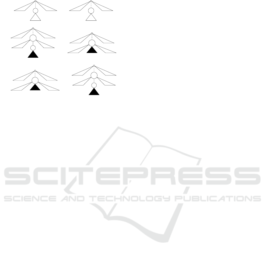
Deﬁnition 2 (Edit operations (Tai, 1979)). The edit

operations of a tree T are deﬁned as follows, see Fig-

ure 1.

1. Substitution: Change the label of the node v in T.

2. Deletion: Delete a node v in T with parent v

′

making the children of v become the children of

′

. The children are inserted in the place of v as a

subsequence in the left-to-right order of the chil-

dren of v

′

. In particular, if v is the root in T, then

the result applying the deletion is a forest consist-

ing of the children of the root.

3. Insertion: The complement of deletion. Insert a

node v as a child of v

′

in T making v the parent of

a consecutivesubsequence a subset of the children

of v

′

Let ε 6∈ Σ denote a special blank symbol and deﬁne

= Σ ∪ {ε}. Then, we represent each edit operation

by (l

7→ l

), where (l

, l

) ∈ (Σ

×Σ

−{(ε, ε)}). The

operation is a substitution if l

6= ε and l

6= ε, a dele-

tion if l

= ε, and an insertion if l

= ε. For nodes v

and w, we also denote (l(v) 7→ l(w)) by (v 7→ w). We

deﬁne a cost function γ : (Σ

× Σ

\ {(ε, ε)}) 7→ R

Computing the Variations of Edit Distance for Rooted Labaled Caterpillars

273

Substitution (v 7→ w)

7→

Deletion (v 7→ ε)

′

7→

′

Insertion (ε 7→ v)

′

7→

′

Figure 1: Edit operations for trees.

pairs of labels. We often constrain a cost function γ to

be a metric, that is, γ(l

, l

) ≥ 0, γ(l

, l

) = 0 iff l

= l

γ(l

, l

) = γ(l

, l

) and γ(l

, l

) ≤ γ(l

, l

)+γ(l

, l

). In

particular, we call the cost function that γ(l

, l

) = 1

if l

6= l

a unit cost function.

Deﬁnition 3 (Edit distance (Tai, 1979)). For a cost

function γ, the cost of an edit operation e = l

7→ l

is given by γ(e) = γ(l

, l

). The cost of a sequence

E = e

, . . . , e

of edit operations is given by γ(E) =

∑

i=1

γ(e

). Then, an edit distance τ

TAI

, T

) be-

tween trees T

and T

is deﬁned as follows:

TAI

, T

) = min







γ(E)



E is a sequence

of edit operations

transforming T

to T







Deﬁnition 4 (Tai mapping (Tai, 1979)). Let T

and

be trees. We say that a triple (M, T

, T

) is a Tai

mapping (a mapping, for short) from T

to T

if M ⊆

V(T

) ×V(T

) and every pair (v

, w

) and (v

, w

) in

M satisﬁes the following conditions.

1. v

= v

iff w

= w

(one-to-one condition).

2. v

≤ v

iff w

≤ w

(ancestor condition).

We will use M instead of (M, T

, T

) when there is no

confusion denote it by M ∈ M

TAI

, T

Let M be a mapping from T

to T

. Let I

and J

be the sets of nodes in T

and T

but not in M, that is,

= {v ∈ T

| (v, w) 6∈ M} and J

= {w ∈ T

| (v, w) 6∈

M}. Then, the cost γ(M) of M is given as follows.

γ(M) =

∑

(v,w)∈M

γ(v, w) +

∑

v∈I

γ(v, ε) +

∑

w∈J

γ(ε, w).

Trees T

and T

are isomorphic without labels,

denoted by T

≡

, if there exists a mapping M ∈

TAI

, T

) such that I

= J

0, and isomorphic,

denoted by T

≡ T

, if there exists a mapping M ∈

TAI

, T

) such that I

= J

0 and γ(M) = 0.

Theorem 1. (Tai, 1979) It holds that:

TAI

, T

) = min{γ(M) | M ∈ M

TAI

, T

)}.

Furthermore, we introduce the variations of the

Tai mapping and the edit distance, which are main

topics in this paper.

Deﬁnition 5. Let T and S be trees and suppose that

M ∈ M

TAI

(T, S). We deﬁne M

−

as M \ {r(T), r(S)}.

1. We say that M is a top-down mapping (Chawathe,

1999; Selkow, 1977), which we denote by M ∈

TOP

(T, S), if (par(v), par(w)) ∈ M for every

(v, w) ∈ M

−

2. We say that M is an LCA-preserving mapping (or

degree-2 mapping) (Zhang et al., 1996), which we

denote by M ∈ M

LCA

(T, S) if (v⊔ v

′

, w⊔ w

′

) ∈ M

for every (v, w), (v

′

, w

′

) ∈ M.

3. We say that M is a bottom-up mapping (Valiente,

2001), which we denote by M ∈ M

BOT

(T, S), if

the following condition holds for every(v, w) ∈ M.



∀v

′

∈ T[v]∃w

′

∈ S[w]



′

, w

′

) ∈ M





∧



∀w

′

∈ S[w]∃v

′

∈ T[v]



′

, w

′

) ∈ M





Furthermore, for ◦ ∈ {TOP, LCA, BOT}, we deﬁne the

distance τ

◦

(T, S) between T and S as the minimum

cost of all the mappings in M

◦

(T, S), that is:

◦

(T, S) = min{γ(M) | M ∈ M

◦

(T, S)}.

Here, we call τ

TOP

, τ

LCA

and τ

BOT

a top-down dis-

tance, an LCA-preserving distance and a bottom-up

distance, respectively.

As the time complexityof the variations of the edit

distance in Deﬁnition 5, the following theorem holds,

also see Table 1 in Section 1.

Theorem 2. Let T and S be trees, where n =

max{|T|, |S|} and d = min{d(T), d(S)}

1. The problem of computing τ

TAI

(T, S) is

MAX SNP-hard (Zhang and Jiang, 1994).

This statement also holds even if both T and S are

binary trees or the maximum height of trees is at

most 3 (Akutsu et al., 2013; Hirata et al., 2011).

2. We can compute τ

TOP

(T, S) and τ

LCA

(T, S) in

O(n

d) time (Yamamoto et al., 2014).

3. The problem of computing τ

BOT

(T, S) is

MAX SNP-hard. This statement also holds

even if both T and S are binary trees (Yamamoto

et al., 2014).

It is know the following theorem for caterpillars.

Theorem 3. (Muraka et al., 2018) Let C and

D be caterpillars, where n = max{|C|, |D|} and

λ = min{|lv(C)|, |lv(D)|}. Then, we can compute

TAI

(C, D) in O(n

λ) time under the unit cost func-

tion.

ICPRAM 2022 - 11th International Conference on Pattern Recognition Applications and Methods

274

3 COMPUTING THE

VARIATIONS FOR

CATERPILLARS

Let C and D be caterpillars. We regard a back-

bone bb(C) as a sequence [v

, . . . , v

], where v

r(C) and (v

, v

i+1

) ∈ E(C), and a backbone bb(D)

as a sequence [w

, . . . , w

], where w

= r(D) and

, w

j+1

) ∈ E(D).

Let L

(1 ≤ i≤ n) denote the set of leaves in ch(v

that is, L

= ch(v

)\ {v

i+1

} for 1 ≤ i ≤ n− 1 and L

ch(v

). Also Let K

(1 ≤ j ≤ m) denote the set of

leaves in ch(w

), that is, let K

= ch(w

) \ {w

j+1

} for

1 ≤ j ≤ m− 1 and K

= ch(w

Recall that C[v] denotes the (complete) subcater-

pillar of C rooted at v. Also C(v) denotes the forest

obtained by deleting the root v in C[v]. For a Cater-

pillar C and a subcaterpillar C

′

of C, we denote the

caterpillar obtained by deleting C

′

from C by C \C

′

When designing the algorithm to compute the

variations of edit distance for caterpillars, we use a

multiset of labels on an alphabet Σ. A multiset on Σ is

a mapping S : Σ → N. For a multiset S on Σ, we say

that a ∈ Σ is an element of S if S(a) > 0 and denote it

by a ∈ S (like as a standard set). The cardinality of S,

denoted by |S|, is deﬁned as

∑

a∈Σ

S(a).

Let S

and S

be multisets on Σ. Then, we

deﬁne the intersection S

⊓ S

, the union S

⊔ S

and the difference S

\ S

as multisets satisfying

that (S

⊓S

)(a) = min{S

(a), S

(a)}, (S

⊔S

)(a) =

max{S

(a), S

(a)} and (S

\ S

)(a) = max{S

(a) −

(a), 0} for every a∈ Σ. Note that S

= S

\(S

⊓

) and |S

\ S

| = |S

\ (S

⊓ S

)| = |S

| − |S

⊓ S

We can compute the edit distance µ between mul-

tisets S and S

′

in O(|S| + |S

′

|) time, since µ(S, S

′

) =

max{|S\ S

′

|, |S

′

\ S|} under the unit cost function (cf.,

(Ukita et al., 2021)).

Let S be a set of vertices. Then, we denote the

multiset of labels on Σ occurring in S by

S. Also, we

denote

∑

v∈S

γ(v, ε) by del(S) and

∑

w∈S

γ(ε, w) by ins(S).

3.1 Top-down Distance

First, we consider the equation to compute the top-

down distance τ

TOP

(C, D) between caterpillars C and

D, illustrated in Figure 2.

Theorem 4. Let C and D be caterpillars, where n =

max{|C|, |D|}. Then, we can compute τ

TOP

(C, D) in

O(n) time under the unit cost function.

Proof. First, we show that the equations in Figure 2

is correct. Suppose that M ∈ M

TOP

(C, D). Note

that bb(C) = [v

, . . . , v

] and bb(D) = [w

, . . . , w

TOP

(C, D) =

min{n,m}−2

∑

i=1



γ(v

, w

) + µ(

)



+ d

n,m

(C, D),

n,m

(C, D) =











γ(v

m−1

, w

m−1

min

(

γ(v

, w

) + µ(

ch(v

) + del(C(v

m+1

)),

µ(

ch(v

m−1

ch(w

m−1

)) + del(C(v

)) + ins(K

)

if n > m,

γ(v

n−1

, w

n−1

min

(

γ(v

, w

) + µ(

µ(

ch(v

n−1

ch(w

n−1

)) + del(L

) + ins(K

)

if n = m,

γ(v

n−1

, w

n−1

min

(

γ(v

, w

) + µ(

ch(w

)) + ins(D(w

n+1

)),

µ(

ch(v

n−1

ch(w

n−1

)) + ins(D(w

)) + del(L

)

if n < m.

Figure 2: The equations of computing τ

TOP

It is obvious that (v

, w

) ∈ M. Also, if (v

, w) ∈

M (resp., (v, w

) ∈ M), then it holds that w = w

(resp., v = v

). Hence, there exists an index h such

that 1 ≤ h ≤ min{n, m} and M contains the pairs

, w

), . . . , (v

, w

). Furthermore, if M is the mini-

mum cost, then M contains the pairs (v

, w

) as many

as possible, so such an h is min{n, m} and such an M

implies τ

TOP

(C, D).

For every i (1 ≤ i ≤ h − 2), we can compute the

correspondences in M between the leaves in L

and

the leaves in K

as µ(

), where

⊓

implicitly

represents such correspondences. Then, it holds that

TOP

(C \ C[h], D \ D[h]) =

h−2

∑

i=1



γ(v

, w

) + µ(

)



which is computed in the formula of τ

TOP

(C, D) ex-

cept d

n,m

(C, D) in Figure 2.

Consider the case that i = h − 1, that is, consider

the formula d

n,m

(C, D).

If n = m, then we can compute

TOP

(C[v

n−1

], D[v

n−1

]) as the sum of γ(v

n−1

, w

n−1

)

and the minimum value of γ(v

, w

) + µ(

) (if v

is corresponding to w

) and µ(

ch(v

n−1

ch(w

n−1

)) +

del(L

) + ins(K

) (otherwise), which is realized as

the second formula in d

n,m

(C, D) in Figure 2.

Suppose that n > m. Then, we can compute

TOP

(C[v

n−1

], D[v

n−1

]) as the sum of γ(v

m−1

, w

m−1

)

and the minimum value of the upper and the lower

formulas in the ﬁrst formula in d

n,m

(C, D) in Figure 2.

If v

is corresponding to w

, then its cost is

γ(v

, w

) and the leaves in K

are possible to cor-

respond to not only the leaves in L

but also v

m+1

that is, ch(v

). Such correspondences are computed

as µ(

ch(v

). Furthermore, the remained ver-

tices in C(v

m+1

) are deleted, which is realized as

Computing the Variations of Edit Distance for Rooted Labaled Caterpillars

275

del(C(v

m+1

)). Hence, the upper formula is correct.

Otherwise, that is, if v

is not corresponding to

, then the vertices in ch(v

m−1

) are correspondingto

the vertices in ch(w

m−1

). Such correspondences are

computed as µ(

ch(v

m−1

ch(w

m−1

)). Furthermore,

the remained vertices in C(v

) are deleted and the re-

mained vertices in K

are inserted, which is realized

as del(C(v

)) + ins(K

). Hence, the lower formula is

correct. Therefore, the ﬁrst formula is correct.

Similarly, for the case that n < m, the third for-

mula in d

n,m

(C, D) in Figure 2 is also correct.

Since the equations traverse at most once for every

vertex in C and D with traversing (v

, w

) and the pro-

cessing for (v

, w

) runs in O(1) time, the total running

time is O(|C| + |D|) = O(n).

3.2 LCA-preserving Distance

Next, we consider the recurrences of computing the

LCA-preserving distance τ

LCA

(C, D) between cater-

pillars C and D illustrated in in Figure 3. Here, we

regard

C[v

i+1

] and

D[w

j+1

] in the recurrences as the

multisets of labels occurring in all the vertices in

C[v

i+1

] and D[w

j+1

LCA

(C[v

], D[w

]) =

min







γ(v

, w

) + µ(

) + τ

LCA

(C[v

i+1

], D[w

j+1

]),

γ(v

, ε) + del(L

) + τ

LCA

(C[v

i+1

], D[w

]),

γ(ε, w

) + ins(K

) + τ

LCA

(C[v

], D[w

j+1

])







if 1 ≤ i < n and 1 ≤ j < m,

LCA

(C[v

], D[w

]) =

min











γ(ε, w

) + ins(K

) + τ

LCA

(C[v

], D[w

j+1

]),

γ(v

, w

)

+ min

v∈L

µ(

{v},

) + µ(

{v},

D[w

j+1

])

γ(v

, w

) + µ(

) + ins(D[w

j+1

])











if 1 ≤ j < m,

LCA

(C[v

], D[w

]) =

min











γ(v

, ε) + del(L

) + τ

LCA

(C[v

i+1

], D[w

]),

γ(v

, w

)

+ min

w∈K

µ(

{w}) + µ(

C[v

i+1

{w})

γ(v

, w

) + µ(

) + del(C[v

i+1

])











if 1 ≤ i < n,

LCA

(C[v

], D[w

]) = γ(v

, w

) + µ(

Figure 3: The recurrences of computing τ

LCA

We start the following simple lemma.

Lemma 1. Let C be a caterpillar. For distinct vertices

v, w ∈ C, it holds that v⊔ w ∈ bb(C).

Proof. If v ∈ bb(C) and w ∈ bb(C), then it holds that

v⊔ w = v or w, which implies that v ⊔ w ∈ bb(C). If

v ∈ bb(C) and w ∈ lv(C), then it holds that v ⊔ w =

v⊔ par(w), which implies that v⊔ w ∈ bb(C). By the

same reason, it holds that v⊔ w ∈ bb(C) if v ∈ lv(C)

and w ∈ bb(C). If v ∈ lv(C) and w ∈ lv(C), then it

holds that v⊔w = par(v)⊔par(w), which implies that

v⊔ w ∈ bb(C).

Theorem 5. Let C and D be caterpillar, where n =

max{|C|, |D|}. Then, we can compute τ

LCA

(C, D) in

O(n

) time under the unit cost function.

Proof. The ﬁrst recurrence in Figure 3 computes that,

for M ∈ M

LCA

(C, D), (1) if (v

, w

) ∈ M, then (v, w) ∈

× K

such that v, w ∈

⊓

are added to M and

next it computes τ

LCA

(C[v

i+1

], D[w

j+1

]), (2) if v

deleted, then all the leaves in L

are deleted and next

it computes τ

LCA

(C[v

i+1

], D[w

]), or (3) if w

is in-

serted, then all the leaves in K

are inserted and next

it computes τ

LCA

(C[v

], D[w

j+1

]), for 1 ≤ i < n and

1 ≤ j < m. Then, the pairs added to M are obtained

from just the case (1), and the pairs consist of some

(v, w) ∈ L

× K

and (v

, w

). Since par(v) = v

and

par(w) = w

and by Lemma 1, M is LCA-preserving.

By the same reason, the mapping obtained from

the last recurrence in Figure 3 is LCA-preserving.

Consider the second recurrence in Figure 3, that

is, the case that τ

LCA

(C[v

], D[w

]) for 1 ≤ j < m and

M ∈ M

LCA

(C, D). The ﬁrst formula means to insert

and L

, and next compute τ

LCA

(C[v

], D[w

j+1

]), no

pairs are added to M.

The second and third formulas mean to add

, w

) to M. Then, the second formula means that

some v ∈ L

is corresponding to some vertex w ∈

D[w

j+1

] (and (v, w) is added to M and the remained

vertices in D[w

j+1

] are inserted), and then L

\ {v} is

corresponding to K

as possible (and the correspond-

ing pairs are added to M). On the other hand, the

third formula means that no v ∈ L

is corresponding

to D[w

j+1

]. In this case, L

is corresponding to K

possible (and the corresponding pairs are added to M)

and the vertices in D[w

j+1

] are inserted.

For both formulas, by Lemma 1, it holds that

⊔ v

, w

⊔ w

) = (v

, w

j+1

) ∈ M for distinct pairs

, w

), (v

, w

) ∈ M∩(C[v

]×D[w

j+1

]). Then, M is

LCA-preserving.

By the same reason, the mapping obtained from

the third recurrence in Figure 3 is LCA-preserving.

Hence, the mapping obtained from the recurrences

in Figure 3 is LCA-preserving.

By traversing C and D at once in O(n) time, we

can obtain the information of v

, w

, L

and K

. Then,

in computing τ

LCA

(C[v

], D[w

]) for a ﬁxed i and j, the

running time is O(1). Since the recurrences compute

LCA

(C[v

], D[w

]) for 1 ≤ i ≤ n and 1 ≤ j ≤ m, the

total running time is O(n

ICPRAM 2022 - 11th International Conference on Pattern Recognition Applications and Methods

276

3.3 Bottom-up Distance

When considering the algorithm of computing the

bottom-up distance τ

BOT

(C, D) between caterpillars C

and D, we deal with the reversal of backbones, that

is, bb(C) = [v

, . . . , v

] for and bb(D) = [w

, . . . , w

where r(C) = v

, (v

, v

i+1

) ∈ E(C), r(D) = w

and

, w

j+1

) ∈ E(D). Then, we design the algorithm

BOTCAT in Algorithm 1.

procedure BOTCAT(C, D)

/* C, D: caterpillars */

/* bb(C) = [v

, . . . , v

], r(C) = v

/* bb(D) = [w

, . . . , w

], r(D) = w

for h = 1 to min{n, m} do1

if |L

| 6= |K

| then break;2

; /* |L

| = |K

| for 1 ≤ i ≤ h */3

A ← bb(C); B ← bb(D); L ← lv(C); K ← lv(D);4

d ← µ(

K) + del(A) + ins(B);5

if h > 0 then6

← d; L

′

← L; K

′

← K;7

for i = 1 to h do8

′

← L

′

i−1

\ L

; K

′

← K

′

i−1

\ K

;

←10

i−1

− γ(v

, ε) − γ(ε, w

) + γ(v

, w

) −

µ(

′

i−1

]

′

i−1

) + µ(

′

);

d ← min{d, d

};11

return d;12

Algorithm 1: BOTCAT.

Theorem 6. Let C and D be caterpillars, where n =

max{|C|, |D|}. Then, we can compute τ

BOT

(C, D) in

O(n) time under the unit cost function.

Proof. Since C and D are caterpillars, if |L

| = |K

for 1 ≤ i ≤ h but |L

h+1

| 6= |K

h+1

|, then it holds that

C[v

] ≡

D[w

] but C[v

h+1

] 6≡

D[w

h+1

]. The algo-

rithm BOTCAT ﬁrst ﬁnds such an h in lines 1, 2 and

3. In this case, we can obtain bottom-up mapping

M ∈ M

BOT

(C, D) between C[w

] and D[w

] by (1)

adding (v

, w

) to M, (2) adding (v, w) to M for v ∈ L

w ∈ K

and l(v) = l(w) and (3) adding (v, w) to M for

the remained v ∈ L

and w ∈ K

for 1 ≤ i ≤ h. We can

compute the distance concerned with the above (2)

and (3) as µ(

). Note that the remained vertices

in C are deleted and those in D are inserted.

After obtaining the above h, the algorithm BOT-

CAT computes the bottom-up distance whose bottom-

up mapping M ∈ M

BOT

(C, D) contain no pair in

bb(C) × bb(D) as d in line 6. Then, in for-loop in

lines from 7 to 12, the algorithm BOTCAT updates d

as the minimum value of the current d and the newly

obtained d

such that (v

, w

) ∈ M. Here, d

is the dis-

tance that v

∈ bb(C) is corresponding to w

∈ bb(D),

by adding γ(v

, w

) instead of γ(v

, ε)+ γ(ε, w

), and L

are corresponding to K

, by adding µ(

) instead

of µ(

′

i−1

′

i−1

). This is realized at line 11, that is, by

using the following formula.

← d

i−1

− γ(v

, ε) − γ(ε, w

) + γ(v

, w

)

−µ(

′

i−1

]

′

i−1

) + µ(

′

In other words, for 1 ≤ i ≤ h, the bottom-up mapping

M ∈ M

BOT

(C, D) is updated by adding (v

, w

) and

the correspondence between L

and K

to M for every

i, after removing the correspondences between L

∪

··· ∪ L

and K

∪ ··· ∪ K

in M. Hence, the algorithm

BOTCAT is correct.

By traversing C and D at once in O(n) time, we

can obtain the information of bb(C), bb(D), lv(C) and

lv(D) (so v

, w

, L

and K

). Then, each of lines 2, 4,

5, 7 and 9 to 11 runs in O(1) time. Hence, the total

running time of the algorithm BOTCAT is O(n).

4 EXPERIMENTAL RESULTS

In this section, we give the experimental results of

computing τ

TOP

, τ

LCA

and τ

BOT

. Here, the computer

environment is that OS is Ubuntu 14.04.6, CPU is In-

tel Xeon E5-1650 v3(3.50GHz) and RAM is 15GB.

We deal with caterpillars for N-glycans from

KEGG

, the largest 5,154 caterpillars (0.1%) in dblp

(refer to dblp

0.1%

), SwissProt and non-isomorphic

caterpillars in TPC-H (refer to TPC-H

◦

) from UW

XML Repository

. Also we deal with caterpillars

obtained by deleting the root in Auction (refer to

Auction

−

) and non-isomorphic caterpillars obtained

by deleting the root in Nasa (refer to NASA

−

◦

Protein (refer to Protein

−

◦

) and University (refer to

University

−

◦

) from UW XML Repository. Table 2 il-

lustrates the information of such caterpillars. Here,

#, n, d, h, λ and β are the number of caterpillars, the

average number of vertices, the average degree, the

average height, the average number of leaves and the

average number of labels.

Then, we use all the pairs in the caterpillars in Ta-

ble 2, of which the number is

#× (#− 1)

. Table 3

illustrates the number (#pairs) of all the pairs in cater-

pillars in Table 2.

Table 4 illustrates the running time to compute

TOP

, τ

LCA

and τ

BOT

, as comparing with τ

TAI

by the

algorithm in (Muraka et al., 2018).

Kyoto Encyclopedia of Genes and Genomes,

http://www.kegg.jp/

http://dblp.uni-trier.de/

http://aiweb.cs.washington.edu/research/projects/xmltk/

xmldata/www/repository.html

Computing the Variations of Edit Distance for Rooted Labaled Caterpillars

277

Table 2: The information of caterpillars.

data # n d h λ β

N-glycans 514 6.40 1.84 4.22 2.18 4.50

dblp

0.1%

5,154 41.74 40.73 1.01 40.73 10.61

SwissProt 6,804 35.10 24.96 2.00 33.10 16.79

TPC-H

◦

8 8.63 7.63 1.00 7.63 8.63

Auction

−

259 4.29 3.00 0.71 3.57 4.29

Nasa

−

◦

33 7.27 5.15 1.64 5.64 3.18

Protein

−

◦

5,150 4,97 3.63 1.16 3.81 4.57

University

−

◦

26 1.35 0.35 0.19 1.15 1.35

Table 3: The number (#pairs) of all the pairs in caterpillars

in Table 2.

data #pairs

N-glycans 131,841

dblp

0.1%

13,279,281

SwissProt 23,143,806

TPC-H

◦

data #pairs

Auction

−

33,411

Nasa

−

◦

528

Protein

−

◦

13,258,675

University

−

◦

325

Table 4: The running time (sec.) to compute τ

TAI

, τ

TOP

LCA

and τ

BOT

data τ

TAI

TOP

LCA

BOT

N-glycans 753.33 1.23 2,804.82 2.57

dblp

0.1%

7,525.28 343.70 1,505.05 737.96

SwissProt 82,031.10 1,594.42 9,819.62 2,138.54

TPC-H

◦

5.78×10

−3

0.64×10

−3

1.77×10

−3

1.43×10

−3

Auction

−

4.55 0.23 0.87 0.94

Nasa

−

◦

20.93×10

−2

0.34×10

−2

4.91×10

−2

0.57×10

−2

Protein

−

◦

2,055.77 118.20 433.22 327.66

University

−

◦

14.22×10

−3

0.40×10

−3

2.84×10

−3

6.58×10

−3

Table 4 shows that, whereas the time complexity

of computing τ

TOP

is same as that of computing τ

BOT

the running time of computing τ

TOP

is slightly smaller

than that of computing τ

BOT

. On the other hand, the

running time of computing τ

LCA

is smaller than that of

computing τ

TAI

except N-glycan. The reason is that

the depth of caterpillars in N-glycan is much larger

than other caterpillars.

Table 5 illustrates the number (#cases) of cases

that τ

TAI

< τ

TOP

, τ

TAI

< τ

LCA

and τ

TAI

< τ

BOT

with their

ratios (%) in all the pairs (#pairs), where “max.” is the

maximum difference from τ

TAI

. Since it always holds

LCA

≤ τ

TOP

, we omit the cases that τ

TAI

< τ

LCA

in Ta-

ble 5 when the number of cases that τ

TAI

< τ

TOP

is 0.

Table 5 show that, for caterpillars in dblp

0.1%

TPC-H

◦

, Auction

−

and University

−

◦

, τ

TOP

is an alter-

native and much faster distance to τ

TAI

. Also, whereas

LCA

is an improved distance of τ

TOP

for caterpillars

in N-glycans, τ

LCA

and τ

TOP

are not changed for the

Table 5: The number (#cases) of cases that τ

TAI

< τ

TOP

TAI

< τ

LCA

and τ

TAI

< τ

BOT

with their ratios (%) in all the

pairs (#pairs) with the maximum difference (max.)

TAI

< τ

TOP

data #pairs #cases % max.

N-glycans 131,841 64,467 48.90 10

dblp

0.1%

13,279,281 0 0.00 0

SwissProt 23,143,806 5,933,179 25.64 30

TPC-H

◦

28 0 0 0

Auction

−

33,411 0 0 0

Nasa

−

◦

528 104 19.70 9

Protein

−

◦

13,258,675 697,697 5.26 50

University

−

◦

325 0 0 0

TAI

< τ

LCA

data #pairs #cases % max.

N-glycans 131,841 5,490 4.16 2

SwissProt 23,143,806 5,933,179 25.64 29

Nasa

−

◦

528 56 10.61 1

Protein

−

◦

132,586,75 348,119 2.63 10

TAI

< τ

BOT

data #pairs #cases % max.

N-glycans 131,841 117,657 89.24 16

dblp

0.1%

13,279,281 12,667,501 95.39 4

SwissProt 23,143,806 23,019,607 99.46 4

TPC-H

◦

28 27 96.43 2

Auction

−

33,411 4,107 12.29 1

Nasa

−

◦

528 403 76.33 4

Protein

−

◦

13,258,675 8,828,524 66.59 5

University

−

◦

325 5 1.54 1

other caterpillars. Furthermore, τ

BOT

is insufﬁcient

to approximate to τ

TAI

since the number of cases that

TAI

< τ

BOT

are much larger than the number of cases

that τ

TAI

< τ

TOP

On the other hand, by focusing on the maxi-

mum difference, for caterpillars in SwissProt and

Protein

−

◦

, the maximum difference of τ

BOT

− τ

TAI

much smaller than that of τ

TOP

− τ

TAI

and τ

LCA

− τ

TAI

Then, for these caterpillars, whereas the number of

cases that τ

TAI

< τ

BOT

is larger than the number of

cases that τ

TAI

< τ

TOP

and τ

TAI

< τ

LCA

, τ

BOT

is more

appropriate to characterize the forms of caterpillars

than τ

TOP

and τ

LCA

In order to improve the results in Table 5, Table 6

summarizes the case that min{τ

TOP

, τ

BOT

By comparing with Table 5, Table 6 shows that

the usage of min{τ

TOP

, τ

BOT

} succeeds to decrease the

maximum difference with slightly decreasing the ra-

tio. Hence, min{τ

TOP

, τ

BOT

} provides to fast approxi-

mate to τ

TAI

for caterpillars.

Finally, we compare the algorithms in this paper

ICPRAM 2022 - 11th International Conference on Pattern Recognition Applications and Methods

278

Table 6: The number (#cases) of cases that τ

TAI

min{τ

TOP

, τ

BOT

} with their ratios (%) in all the pairs

(#pairs) with the maximum difference (max.).

data #pairs #cases % max.

N-glycans 131,841 59,921 45.45 9

dblp

0.1%

13,279,281 0 0.00 0

SwissProt 23,143,806 5,933,179 25.64 2

TPC-H

◦

28 0 0 0

Auction

−

33,411 0 0 0

Nasa

−

◦

528 94 17.80 1

Protein

−

◦

13,258,675 637,773 4.81 2

University

−

◦

325 0 0 0

for caterpillars with the algorithms designed by (Ya-

mamoto et al., 2014) for standard trees. Table 7 illus-

trates the running time of computing τ

TOP

and τ

LCA

using such algorithms which refer to τ

TOP

and τ

LCA

Here, “–” denotes time out over 10,000 seconds.

Table 7: The running time (sec.) of computing τ

TOP

and

LCA

by using the algorithms in this paper and the algo-

rithms τ

TOP

and τ

LCA

in (Yamamoto et al., 2014).

data τ

TOP

LCA

TOP

LCA

N-glycans 1.23 2,804.82 11.77 25.64

dblp

0.1%

343.70 1,505.05 – –

SwissProt 1,594.42 9,819.62 – –

TPC-H

◦

0.64×10

−3

1.77×10

−3

3.77×10

−3

7.45×10

−3

Auction

−

0.23 0.87 1.20 2.12

Nasa

−

◦

0.34×10

−2

4.91×10

−2

5.64×10

−2

10.68×10

−2

Protein

−

◦

118.20 433.22 628.79 1156.32

University

−

◦

0.40×10

−3

2.84×10

−3

2.93×10

−3

2.19×10

−3

Table 7 shows that the algorithm of computing

TOP

in this paper is much faster than τ

TOP

. Also,

except N-glycans and University

−

◦

, the algorithm of

computing τ

LCA

in this paper is faster than τ

LCA

5 CONCLUSION

In this paper, we have designed the algorithms of

computing τ

TOP

and τ

BOT

for caterpillars in O(n) time

and τ

LCA

in O(n

) time. Also, we have given ex-

perimental results of computing τ

TOP

, τ

LCA

and τ

BOT

for caterpillars in real data. Then, the usage of

min{τ

TOP

, τ

BOT

} have provided to fast approximate to

TAI

for caterpillars. Also, the algorithms in this pa-

per have been almost fast and faster than the previous

algorithms for trees (Yamamoto et al., 2014).

Since the algorithm of computing τ

LCA

for cater-

pillars is slow for N-glycan, it is a future work to im-

prove the implementation, in particular, to apply to

larger number of caterpillars such as all-glycans in

KEGG and CSLOGS

. Also it is a future work to in-

vestigate the other variations of the edit distance for

caterpillars presented in (Yoshino and Hirata, 2017).

REFERENCES

Akutsu, T., Fukagawa, D., Halld´orsson, M. M., Takasu, A.,

and Tanaka, K. (2013). Approximation and parame-

terized algorithms for common subtrees and edit dis-

tance between unordered trees. Theoret. Comput. Sci.,

470:10–22.

Chawathe, S. S. (1999). Comparing hierarchical data in ex-

ternal memory. In Proc. VLDB’99, pages 90–101.

Deza, M. M. and Deza, E. (2016). Encyclopedia of dis-

tances (4th ed.). Springer.

Gallian, J. A. (2007). A dynamic survey of graph labeling.

Electorn. J. Combin., 14:DS6.

Hirata, K., Yamamoto, Y., and Kuboyama, T. (2011). Im-

proved MAX SNP-hard results for ﬁnding an edit dis-

tance between unordered trees. In Proc. CPM’11

(LNCS 6661), pages 402–415.

Kuboyama, T. (2007). Matching and learning in trees. Ph.D

thesis, University of Tokyo.

Muraka, K., Yoshino, T., and Hirata, K. (2018). Computing

edit distance between rooted labeled caterpillars. In

Proc. FedCSIS’18, pages 245–252.

Selkow, S. M. (1977). The tree-to-tree editing problem. In-

form. Process. Lett., 6:184–186.

Tai, K.-C. (1979). The tree-to-tree correction problem. J.

ACM, 26:422–433.

Ukita, Y., Yoshino, T., and Hirata, K. (2021). Caterpil-

lar alignment distance for rooted labeled caterpillars:

Distance based on alignments required to be caterpil-

lars. In Recent advance in computational optimiza-

tion, pages 111–134.

Valiente, G. (2001). An efﬁcient bottom-up distance be-

tween trees. In Proc. SPIRE’01, pages 212–219.

Yamamoto, Y., Hirata, K., and Kuboyama, T. (2014).

Tractable and intractable variations of unordered tree

edit distance. Internat. J. Found. Comput. Sci.,

25:307–329.

Yoshino, T. and Hirata, K. (2017). Tai mapping hierarchy

for rooted labeled trees through common subforest.

Theory of Comput. Sys., 60:769–787.

Zhang, K. and Jiang, T. (1994). Some MAX SNP-hard re-

sults concerning unordered labeled trees. Inform. Pro-

cess. Lett., 49:249–254.

Zhang, K., Wang, J., and Shasha, D. (1996). On the editing

distance between undirected acyclic graphs. Internat.

J. Found. Comput. Sci., 7:43–58.

http://www.cs.rpi.edu/˜zaki/www-

new/pmwiki.php/Software/Software

Computing the Variations of Edit Distance for Rooted Labaled Caterpillars

279