Enhanced Local Gradient Smoothing: Approaches to Attacked-region

Identiﬁcation and Defense

Cheng You-Wei and Wang Sheng-De

Department of Electrical Engineering, National Taiwan University, Taipei, Taiwan

Keywords:

Adversarial Attack, Adversarial Defense, Reactive Defense, Data Pre-processing, Deep Learning.

Abstract:

Mainstream deep learning algorithms have been shown vulnerable to adversarial attacks - the deep models

could be misled by adding small unnoticeable perturbations to the original input image. These attacks could

pose security challenges in real-world applications. The paper focuses on how to defend against an adversarial

patch attack that conﬁnes such noises within a small and localized patch area. We will discuss how an ad-

versarial sample affects the classiﬁer output from the perspective of a deep model by visualizing its saliency

map. On the basis of our baseline method: Local Gradients Smoothing, we further design two methods

called Saliency-map-based Local Gradients Smoothing and Weighted Local Gradients Smoothing, integrating

saliency maps with local gradient maps to accurately locate a possible attacked region and perform smooth-

ing accordingly. Experimental results show that our proposed method could reduce the probability of false

smoothing and increase the overall accuracy signiﬁcantly.

1 INTRODUCTION

In recent years, deep neural architectures have

achieved signiﬁcant success in most computer vision

ﬁelds, including Image Classiﬁcation, Object Detec-

tion, and face recognition. Convolutional Neural Net-

works (CNNs) became prominent among different ar-

chitectures due to their ability to extract image fea-

tures. Those methods also had been widely applied

to real-world systems like surveillance cameras and

autonomous driving (Huval et al., 2015). The con-

sistency of the learning-based algorithms is one of

the biggest concerns before adopting deep neural net-

works in security-critical applications.

However, Convolutional Neural Networks

(CNNs) had been proven vulnerable to some

well-designed attack methods. J. Goodfellow et

al. (Goodfellow et al., 2015) showed that by slightly

modifying input data or, in other words, adding

subtle noises onto the original input image(s), CNN

models could wrongly classify the input with high

conﬁdence. These noises should be imperceptible to

humans or should not affect human’s recognition of

the image. An adversarial attack could be roughly

explained as ﬁnding the minimal perturbation which

is strong enough to alternate the position of the input

in space and cross the decision boundary.

Among all works, attacks can be divided into

two categories: traditional attack and patch attack.

Traditional attack FGSM (Goodfellow et al., 2015),

PGD (Madry et al., 2018) and One Pixel Attack (Su

et al., 2019) do not try to limit the size of the adver-

sarial mask; hence the size of adversarial perturba-

tions can be as large as the target image. However,

even with remarkable success on benchmarks, in real-

world scenarios, there might be some obstacles in ap-

plying those perturbations onto real objects. While

patch attack conﬁnes the perturbations in a small area,

those patches can be used as stickers in real-world

scenarios. Image patches generated by Adversarial

Patch (Brown et al., 2017) can cause a classiﬁer to

output any target class and can be printed and added to

any scene. Afterward, LaVAN (Karmon et al., 2018)

will successfully conﬁne the patch to a small, local-

ized patch of the image without covering any of the

main objects and fool the state-of-the-art classiﬁer In-

ceptionv3 (Szegedy et al., 2016).

Applications of the above methods vary in many

parts of life. DPatch (Liu et al., 2019) can fool object

detectors like YOLO and Faster-RCNN with a 40*40

patch. Based on DPatch (Liu et al., 2019), Physical

Adversarial Patches (Lee and Kolter, 2019) fails hu-

man detectors by drawing all attention to the patch

itself. Instead of failing the whole system, Simen

Thys et al. innovated a method (Thys et al., 2019)

254

You-Wei, C. and Sheng-De, W.

Enhanced Local Gradient Smoothing: Approaches to Attacked-region Identiﬁcation and Defense.

DOI: 10.5220/0010825400003116

In Proceedings of the 14th International Conference on Agents and Artiﬁcial Intelligence (ICAART 2022) - Volume 2, pages 254-263

ISBN: 978-989-758-547-0; ISSN: 2184-433X

that only makes the person holding cardboard in front

of the body undetectable by YOLOv2. In addition to

malicious usage, Adversarial CAPTCHAs (Shi et al.,

2021) and Robust Text CAPTCHAs (Shao et al.,

2021) address a more secure CAPTCHA (Completely

Automated Public Turing test to tell Computers and

Humans Apart) with adversarial examples.

Defense against adversarial samples had become

an important security issue. Reactive methods typ-

ically remove adversarial noises by applying sets of

transformations. Simple ﬁlters including median and

Gaussian are cheap but perform poorly against strong

attacks. Moreover, these simple ﬁlters can be de-

tected by attackers and then used to optimize attack

methods accordingly. Ensemble Defense with Data

Diversity (Li et al., 2021) ensembles a set of ﬁlters

with high diversity to satisfy randomness and repre-

sentation and thus augment the performance. How-

ever, these methods against adversarial attacks do not

ﬁt well in defending adversarial patch attacks. Since

the noise is concentrated on a small patch area, it is

unnecessary and in conductive to apply a ﬁlter onto

the whole image. On the contrary, we believe a de-

fense mechanism consisting of detection and defense

stage will be more effective against adversarial patch

attacks. In this paper, we introduce an evolved de-

fensive scheme based on a previous work called Lo-

cal Gradient Smoothing (Naseer et al., 2019) to detect

and remove adversarial noises according to the result

of an attack-region proposing module. This method

does not require changing either the architecture of

the deep neural network or the parameters. Instead, it

works in the preprocessing stage that modiﬁes input

data with some smoothing mechanisms. The contri-

butions of this paper can be summarized as follows:

1) By investigating the adversarial phenomena, we

visualize how the perception of the deep model

changes while given an adversarial sample in con-

trast to a normal input, also showing how differ-

ent CNN architectures and different experimental

settings affect the inﬂuence of adversarial attack

methods.

2) Motivated by our baseline method (Naseer et al.,

2019), which proposes a strategy called Local

Gradients Smoothing (LGS). LGS ﬁrst estimates

the region of interest in the input image of adver-

sarial noise and then performs gradient smoothing

against it. We raise its performance by incorporat-

ing the information of deep visual features, which

is also called the saliency map.

3) We propose two different algorithms: Saliency-

map-based Local Gradients Smoothing (SLGS)

and Weighted Local Gradients Smoothing

(WLGS). Both methods outperform the baseline

method and other top methods such as image

ﬁltering mechanisms, JPEG compression, and

digital watermarking (DW) (Hayes, 2018).

Figure 1: Example images with VGG16 (Simonyan and

Zisserman, 2014) classiﬁcation result and conﬁdence score.

(a) shows the original image sample from (Russakovsky

et al., 2015), (b) is the adversarial sample generated by

LaVAN (Karmon et al., 2018), (c) represents the result of

Saliency-map-based Local Gradients Smoothing (SLGS),

and (d) is the result of Weighted Local Gradients Smooth-

ing (WLGS). As illustrated, both proposed methods suc-

cessfully turned the classiﬁcation result into the correct la-

bel.

2 RELATED WORKS

2.1 Attack Method

Traditional adversarial attack methods aim to ﬁnd ad-

versarial samples by adding some noise to original

inputs. Goodfellow et al. (Goodfellow et al., 2015)

propose a fast and strong method to ﬁnd adversarial

examples. Papernot et al. (Papernot et al., 2016a) use

the saliency map to explain how adversaries are gen-

erated and bring up an attack accordingly. The search

for adversarial examples can be formulated as ﬁnding

a solution x0 to the following equation:

F (y = ¯y|x0)

subject tokx − x0k

≤ ε

(1)

where x0 is the image sample with adversarial noise

added onto the original image x. Instead of limiting

the size of the noise, it restrains the magnitude of the

sum of the noise within a threshold ε. The objective

function of targeted attack is to make the prediction

result of an image classiﬁer F fall into a speciﬁc tar-

get class ¯y, while the value of perturbation remains

within a threshold. Non-targeted attack is formulated

by making the output become any class other than the

original label; hence it is considered easier to achieve

than the targeted attack.

Researchers of Adversarial Patch (Brown et al.,

2017) ﬁnd adversarial examples created using the

methodology presented in the above equation cannot

be used in physical world attacks because adversarial

noise loses its effect under different camera angles,

rotations, and lighting conditions. Brown et al. use a

Enhanced Local Gradient Smoothing: Approaches to Attacked-region Identiﬁcation and Defense

255

variant of the Expectation over Transformation (EoT)

framework to create dependent robust noise patches

conﬁned to a small region that can be printed and

placed in real-world scenarios to cause misclassiﬁca-

tions. They design a patch operator A(p, x, l, t) for a

given image x, patch p, location l and a set of transfor-

mations t. The adversarial patch is obtained by solv-

ing the following optimization problem:

p0 = max

E([F( ¯y|A(p, x, l, t))]) (2)

During optimization, patch operator A applies a

set of transformations to the patch p and then projects

it onto the image x. Finally, the patch p0 has the great-

est expectation over transformations.

Furthermore, LaVAN (Karmon et al., 2018) con-

ﬁnes adversarial noise δ to a small region, usually

away from the salient object in an image. Instead of

training the noise to either maximize the probability

of the target class or to minimize the probability of

any other class, they use a loss function to achieve

both:

x0 = (1 − m)  x + m  δ

argmax

[M(y = ¯y|x0) − M(y = ˆy|x0)]

(3)

where M represents the activations prior to the ﬁnal

softmax layer in the network, ¯y is the target class, and

ˆy is the source class. After training, it uses a spa-

tial mask m to replace the small area with noise, as

opposed to noise addition performed in traditional at-

tacks.

2.2 Defense Method

In the defensive phase, there are also two main cate-

gories: proactive and reactive defense. Proactive de-

fense methods aim to make the model robust to adver-

sarial samples by adjusting the training process. Ad-

versarial Training (Shaham et al., 2015) includes ad-

versarial samples as training data, which reduces the

impact of adversarial perturbations. This data aug-

mentation also leads to a more stable model. De-

fensive Distillation (Papernot et al., 2016b) applies

the technique of knowledge distillation. The process

starts by training a teacher network that will gener-

ate soft labels, then trains a student network to ﬁt

the soft label, which is also the teacher’s probabil-

ity distribution. The student network is the network

that will be used for inference. This method leads

to a smoother decision boundary, making adversar-

ial samples harder to be found by attackers. Car-

lini et al. (Carlini and Wagner, 2017) then propose a

stronger attack against Defensive Distillation (Paper-

not et al., 2016b). Inspired by (Carlini and Wagner,

2017), Papernot et al. (Papernot and McDaniel, 2017)

modify the original mechanism soon. The reactive

defense method, also called transformation-based de-

fense, focuses on detecting and removing adversarial

noises on images before feeding them into convolu-

tion networks. This sort of method does not require

changing any of the DNN architectures. For example,

there are works studying reducing noise with JPEG

and JPG compression (Das et al., 2018) (Dziugaite

et al., 2016). Feature Squeezing (Xu et al., 2017)

applies image ﬁltering techniques, including median

ﬁltering and Gaussian ﬁltering to resist adversarial at-

tacks. Digital Watermarking(DW) (Hayes, 2018) ﬁrst

introduces using the saliency map to detect and de-

fend against attackers. Our baseline method lies un-

der this category. In this paper, we improve one of the

most successful methods: Local Gradients Smooth-

ing (Naseer et al., 2019) by adding another noise de-

tection mechanism in the preprocessing stage. LGS

observes adversarial noise as high-frequency noise,

which can be detected by calculating local gradients.

Details are to be discussed in the next section.

2.3 Baseline Method: Local Gradients

Smoothing: Defense against

Localized Adversarial Attacks

Previous attacks (Brown et al., 2017) (Karmon et al.,

2018) introduce high-frequency noise concentrated at

a particular image location, and such noise becomes

very prominent in the image gradient domain. It

can be observed by the image characteristics of the

patch. The effect of such adversarial noise can be

reduced signiﬁcantly by suppressing high-frequency

regions without affecting the low-frequency image ar-

eas. LGS proposed a method by projecting a gradient

magnitude map onto the image.

LGS obtains the gradient magnitude map by es-

timating the ﬁrst-order local image gradient of each

pixel, which is calculated by the ﬁrst-order partial dif-

ferential of others pixels along in x and y axis. The re-

gions with stronger gradients have a higher likelihood

of being the perturbed areas. The gradient is obtained

by the image’s characteristics only. Hence, they do

not provide signiﬁcant information for the ﬁnal clas-

siﬁcation result. Approaches to estimate the region’s

contribution to the predicted result will be discussed

in the later section. The local gradient of each pixel x

is computed as follows:

∇x(a, b) =

(

∂x

∂a

)

+ (

∂x

∂b

)

(4)

where a and b denotes the horizontal and vertical di-

ICAART 2022 - 14th International Conference on Agents and Artiﬁcial Intelligence

256

rections in the image plane.

They then divide the gradient magnitude map into

K blocks of the same sizes and apply a threshold to

decide whether to keep or remove the block. If the to-

tal value of the local gradient within a block does not

exceed the threshold, the block will be masked out to

zero on the gradient magnitude map. After normal-

ization, the gradient magnitude map g(x) is then used

to suppress the high-frequency parts by performing

“smoothing” to input image:

T (x) = x  (1 − λ ∗ g(x)) (5)

where T (x) is the result after LGS transformation, 

denote element-wise multiplication of two matrices,

and λ is the smooth factor.

3 APPROACH

According to Local Gradients Smoothing

(LGS) (Naseer et al., 2019), one of the impor-

tant control factors is λ, the smoothing factor for

LGS. The smoothing factor decides how much

information will be removed on those regions that are

considered perturbed. Even though LGS masked out

blocks with gradient magnitude below a particular

threshold, it still becomes a trade-off between clean

images and perturbed images in accuracy. If λ is too

small, the defense would fail to smooth out adver-

sarial noises. In large λ cases, LGS could remove

noises but could also remove too much ground-truth

information at the same time, which would lead to

an unexpected result. The image classiﬁer could

classify the image into another class instead of the

ground-truth or the attacking target.

We believe it is necessary to locate the adversar-

ial noises with higher precision, not only from image-

level information but also from what the classiﬁer had

perceived, to make the smoothing process more accu-

rate.

A mathematically clean way of locating “impor-

tant” pixels is to construct a sensitivity map—also

called saliency map—obtained by differentiating

class activation function S with respect to input x. The

saliency map M represents how much difference a

tiny change in each pixel of x would make to the clas-

siﬁcation score for class c. The sensitivity map of a la-

bel will be highly correlated to regions where that la-

bel is present. In practice, the approach is widely used

for the visualization of CNNs. Here we refer to the

implementation of constructing Saliency Maps (Si-

monyan et al., 2013):

(x) =

∂S

∂x

(6)

where M represents the saliency map with the same

shape of the input image, and S

is the ﬁnal class ac-

tivation function of the image classiﬁer.

We design a slightly different version of the sen-

sitivity map. Since the effect of attacks is not always

guaranteed, the target class may not be predicted as

the only possible class; thus it may not be the promi-

nent part on the sensitivity map. Instead of using the

whole class score, we thereby design a loss function

calculating the cross entropy of the top 5 classes.

In most cases where adversarial samples success-

fully fooled the classiﬁer, we will ﬁnd out that the

sensitivity map and the local gradient map highlights

different areas but both cover areas where the adver-

sarial sample is located. One of the na

ıve thoughts

is to ﬁnd the overlapping areas of the two approaches

mentioned above. We propose two ways of integrat-

ing the sensitivity map and the local gradient map to

boost up the accuracy of the attacked-region proposal.

In this paper, we apply the same local gradient map

g(x) presented in LGS (Naseer et al., 2019).

Saliency-map-based Local Gradients Smoothing

(SLGS): we take the primary parts of the saliency

map to perform gradient smoothing, the rest will be

ignored. One possible problem of the saliency map is

that even when there is apparent noise, the pixels are

still scattered. To complete a mask, we take a thresh-

old to binarize the saliency map:

x,y

(

1, if M

x,y

≥ threshold

0, otherwise

(7)

where the threshold is designed as the mean value of

the saliency map M obtained by Eq. 6 in our experi-

ments.

Then we use a combination of erosion and dila-

tion to remove small empty “holes” and clear outliers.

Finally, we multiply element-wise the local gradient

map with the updated saliency mask. If a pixel has a

negative value of the mask, the gradient will be zeroed

out. The operators of binary erosion E and dilation D

based on the binary mask obtained by Eq. 7 with the

kernel size 3 for every pixel (i, j) are deﬁned as fol-

lows:

E(i, j) = M(i, j) ∩ (M(i − 1, j − 1) ∪ M(i − 1, j)

M(i − 1, j + 1) ∪ M(i, j − 1) ∪ M(i, j + 1)

M(i + 1, j − 1) ∪ M(i + 1, j) ∪ M(i + 1, j + 1))

(8)

D(i, j) = E(i, j) ∪ E(i − 1, j − 1) ∪ E(i − 1, j)

E(i − 1, j + 1) ∪ E(i, j − 1) ∪ E(i, j + 1)

E(i + 1, j − 1) ∪ E(i + 1, j) ∪ E(i + 1, j + 1)

(9)

Enhanced Local Gradient Smoothing: Approaches to Attacked-region Identiﬁcation and Defense

257

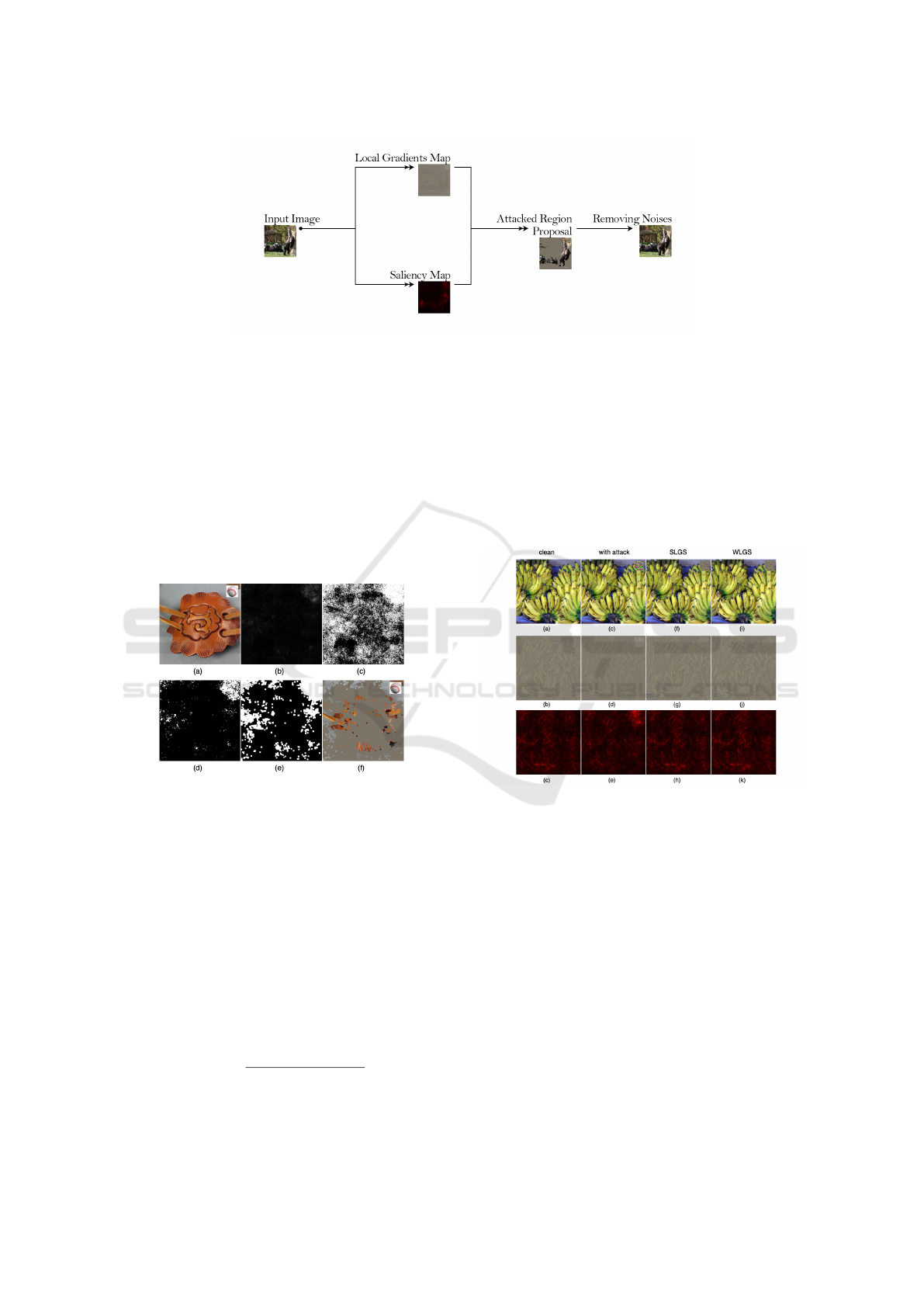
Figure 2: Defense Mechanism.

where ∩ denotes the logical and, i.e.intersection oper-

ation and ∪ denotes the union. In our experiments, we

apply two times of erosion followed by three times of

dilation to form a mask. We then perform the smooth-

ing operation based on the element-wise multiplica-

tion of the ﬁnal dilated mask D(x) along with the local

gradient map g(x) as Eq. 10:

T (x) = x  (1 − λ ∗ D(x)  g(x)) (10)

where  denotes the element-wise multiplication of

two matrices, and λ is a scaling factor, which controls

the intensity of eliminating noises.

Figure 3: Steps for attacked-region proposal using saliency

map. (a) is the original image, (b) represents the saliency

map, (c) is the binary mask of (b), (d) is the mask after

erosion, (e) shows (d) after dilation, and (f) illustrates the

selected regions. The gray areas will be considered as non-

attacked parts.

Weighted Local Gradients Smoothing (WLGS):

there are times when the local gradient map and sen-

sitivity map do not reach an agreement on candidate

regions. Hence, we simply use the saliency map as

the weight matrix for local gradients. The saliency

map varies within a large range, so we normalize it

for consistency among all samples using the follow-

ing equation:

W (x) =

M(x) − M(x)

min

M(x)

max

− M(x)

min

(11)

where we take the normalized map W as the weight

matrix, representing the possibility of containing ad-

versarial noise in each pixel. The ﬁnal gradient map is

obtained by re-weighting the local gradient map with

the weight matrix as Eq. 12:

T (x) = x  (1 − λ ∗ (M(x) ∗ g(x))) (12)

We set the local gradient map threshold = 0.2 and

the saliency map threshold = mean value of the map

and searched a wide range of smooth factors in our

experiments. We further discuss and demonstrate the

advantages of SLGS and WLGS in later sections.

Figure 4: Visualizing changes of the local gradient map and

the saliency map. The ﬁrst row shows the image in human

perception, the second row is the local gradient map, and

the third row illustrates the saliency map.

4 EXPERIMENT

4.1 Experiment Setup

Our proposed methods are evaluated on artiﬁcially

created adversarial masks (Brown et al., 2017) (Kar-

mon et al., 2018) added on ImageNet ILSVRC-

2012 (Simonyan and Zisserman, 2014) dataset. To

compare our methods to the baseline method, we

use identical experimental settings and parameters on

both works. Our experiments can be separated into

two parts: training and testing. For adversarial patch

ICAART 2022 - 14th International Conference on Agents and Artiﬁcial Intelligence

258

generation and Local Gradients Smoothing reproduc-

tion, we refer to the code source: https://github.com\

/metallurk\/local\ gradients\ smoothing.

Training: This part aims to reproduce the results of

Adversarial Patch and LaVAN attacks, creating ro-

bust targeted adversarial patches in the white box set-

ting. Both were trained and validated with the Ima-

geNet ILSVRC 2012 training set with 1000 classes

and more than 1281k images in our experiments on a

single GeForce RTX-2080-ti GPU. Two pre-trained

models, VGG16 (Simonyan and Zisserman, 2014)

and InceptionV3 (Szegedy et al., 2016) were utilized

respectively to experiment on the attack mechanisms.

We use Pytorch (Paszke et al., 2019) framework and

load the pre-trained architecture and weights from

Torchvision. Instead of changing the model weights,

we ﬁx the weights and optimize the patch in input im-

ages by stochastic gradient descent with momentum.

We use the same hyperparameters for both attacks:

Due to the limitation of memory, we set the batch

size to 20 and train size to 50, which means for each

epoch, we sample a new collection of 20*50=1000

images from the dataset. The learning rate is 1 for

the ﬁrst 160 epochs and then decay to 0.1 for 20

epochs, lastly 0.01 for the last 20 epochs, with a total

of 200 epochs. Before feeding images into networks,

we normalize and resize input images to 400x400

size. Three LaVAN masks with size 42x42 (≈1% of

the image), 52x52 (≈1.7% of the image), and 60x60

(≈2.2% of the image) were applied. For Adversarial

Patch, the patch size is 90x90(≈5% of the image).

Testing: To show the improvement of our methods,

we apply the same patch attacks as stated above onto

a subset consisting of 5000 samples from ImageNet

ILSVRC 2012 validation set, which originally has

50000 images in total, and then exploit our proposed

methods and the baseline method to defend against

the attack. For deducing the inconsistency and avoid-

ing the patch covering the salient objects, we always

place the patch on the top-right corner with 10 pixels

away from the corner. Lastly, we simply use top-1

accuracy as the evaluation matrix.

4.2 Experiment Results

For the smoothing factor λ, we found that it is not easy

to give the most suitable value, as different attack-

ers lead to different results, so we searched through

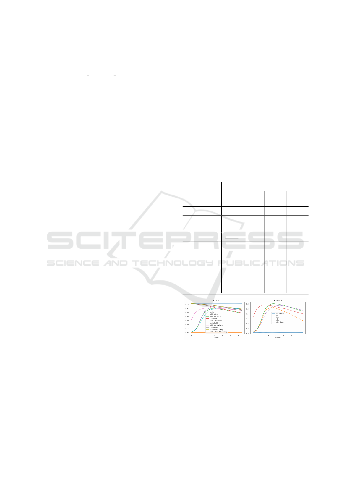
a wide range of lambdas. Table 1 demonstrates the

effect of our proposed method defending against La-

VAN attacks on VGG16, comparing them to the base-

line method with various lambdas. As shown in

Fig. 5, Saliency-map-based Local Gradients Smooth-

ing (SLGS) has signiﬁcant improvements from Lo-

cal Gradients smoothing (LGS), while Weighted Lo-

cal Gradients Smoothing (WLGS) is comparable to

LGS. This is due to the addition of an attacked-region

proposing mechanism to the initial algorithm that re-

duces the probability of false smoothing without sac-

riﬁcing its capability to smooth out most attacks. As

in Fig. 5, we measure the results for both scenar-

ios, with and without attackers, and for readability,

we only take into account the average result for each

scheme.

Table 1: Summary of VGG16 performance against La-

VAN attack with and without defenses including Local Gra-

dients smoothing (LGS), Saliency-map-based Local Gra-

dients Smoothing (SLGS), and Weighted Local Gradients

Smoothing (WLGS). Bold numbers represent the best accu-

racy of a certain defense against LaVAN attack. Underlined

numbers represent the best accuracy of a method among all

smooth factors.

Model VGG16

Patch Size - 42

(1%)

(1.7%)

(2.2%)

No Defense 72.24 0.32 0.48 0.33

LGS(λ=3.5) 64.28 62.32 59.26 54.10

LGS(λ=2.7) 67.74 60.92 50.70 37.98

LGS(λ=2.3) 68.64 55.60 36.48 20.74

WLGS(λ=3.5) 65.42 54.36 63.08 50.12

WLGS(λ=2.7) 67.38 53.02 60.14 47.98

WLGS(λ=2.3) 68.64 51.88 58.68 46.30

SLGS(λ=3.5) 68.20 66.50 63.10 57.08

SLGS(λ=2.7) 69.64 63.68 53.04 39.18

SLGS(λ=2.3) 70.48 57.26 37.70 21.50

Figure 5: Visualizing average top-1 accuracy defending La-

VAN attack on VGG16 with different lambda values among

LGS, SLGS, and WLGS. Patch Size = 52x52. In WLGS

clamp, we clip the value of normalized saliency in (0,1).

Patch Size = 52x52. Left: accuracy with and without at-

tack. Right: average accuracy with and without attack.

As demonstrated in Table 2, which shows the ef-

fect of our proposed method defending against La-

VAN attack on InceptionV3, our proposed methods

do not show any notable improvement as on VGG16,

yet still comparable. The primary reason for the dif-

ference is the dependency on the precision of the

Enhanced Local Gradient Smoothing: Approaches to Attacked-region Identiﬁcation and Defense

259

attacked-region proposal. As InceptionV3 originally

shows more robustness against adversarial samples

without any defenses, the success rate of the targeted

attack drops signiﬁcantly. Table 3 and 4 shows the re-

sult of our proposed method defending against Adver-

sarial attack on VGG16 and InceptionV3 respectively.

The enhancement of SLGS is still over 1.5 percent in

both scenarios, while WLGS drops a lot. We will il-

lustrate some outcomes to show the effect and related

explanations in the subsequent experimental discus-

sion.

Table 2: Summary of InceptionV3 performance against La-

VAN attack with and without defenses.

Model InceptionV3

Patch Size - 42

(1%)

(1.7%)

(2.2%)

No Defense 78.70 12.36 9.96 5.92

LGS(λ=2.3) 77.66 77.40 77.18 76.98

LGS(λ=1.9) 77.88 76.88 77.18 74.70

LGS(λ=1.5) 78.16 71.08 72.26 55.06

WLGS(λ=2.3) 77.46 75.50 77.34 77.22

WLGS(λ=1.9) 78.26 72.20 77.00 75.36

WLGS(λ=1.5) 78.26 64.46 73.64 65.34

SLGS(λ=2.3) 77.88 77.26 77.32 76.82

SLGS(λ=1.9) 78.32 75.88 76.98 74.54

SLGS(λ=1.5) 78.46 68.00 72.12 54.94

Table 3: Summary of VGG16 performance against Adver-

sarial Patch attack with and without defenses. λ=3.5

Model Name VGG16

Method - LGS WLGS SLGS

No Attack 71.70 64.34 64.82 67.38

With Attack 0.12 60.88 24.02 63.36

Table 4: Summary of InceptionV3 performance against Ad-

versarial Patch attack with and without defenses. λ=3.5

Model Name InceptionV3

Method - LGS WLGS SLGS

No Attack 79.56 76.64 77.30 77.38

With Attack 0.10 75.92 65.36 76.46

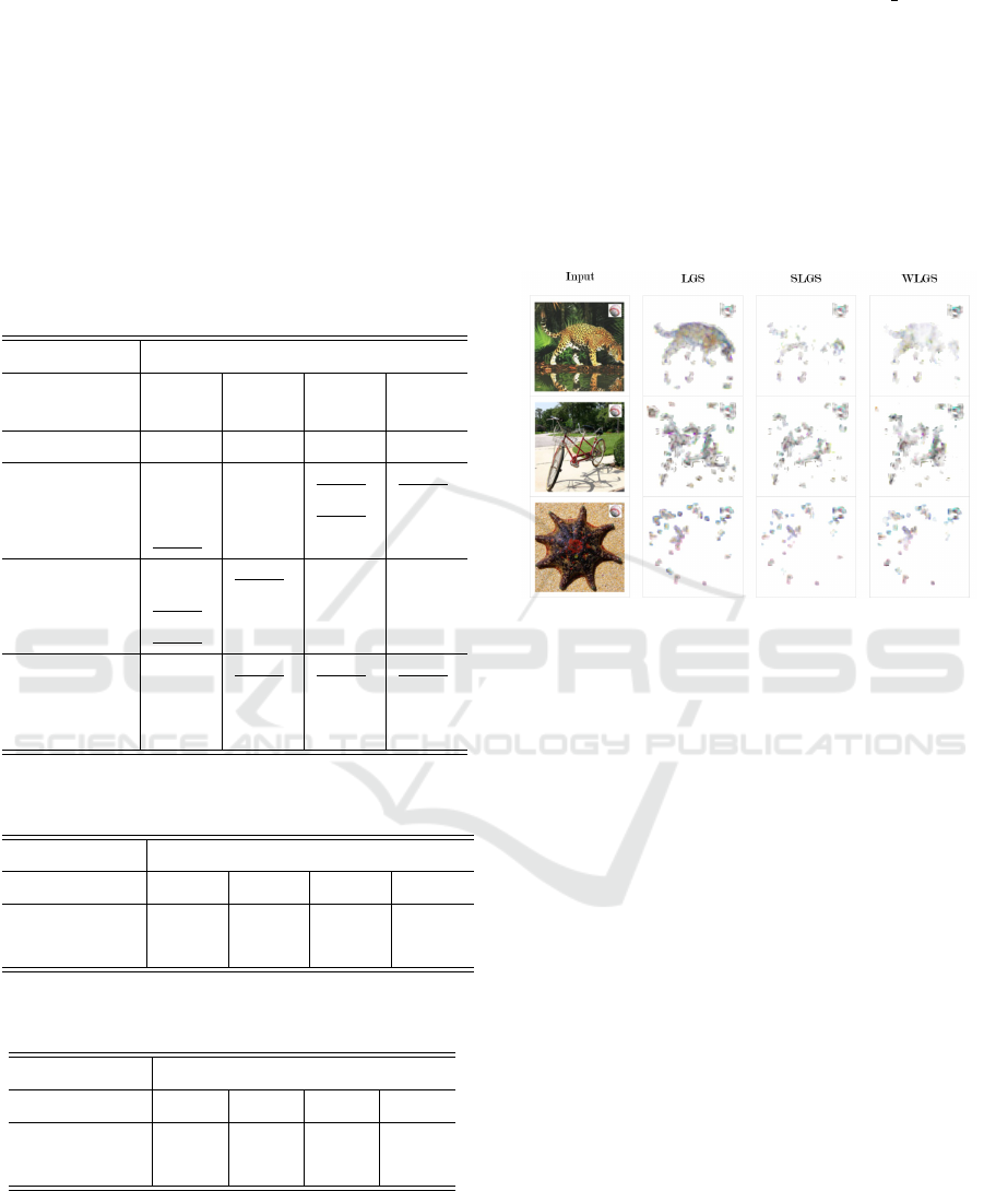
To emphasize the improvement of our proposed

methods compared to the baseline method under the

situation where we successfully decrease the extent of

smoothing out the ground-truth object, we measured

the difference between the input image and the result

after image-preprocessing using structural similarity

from scikit-image. We conduct experiments on a set

of 1000 images computing the average similarity in-

dex between the original input and the output of each

method. As a result, the average similarity index of

LGS is 0.971, SLGS is 0.987, and WLGS is 0.981.

Fig. 6 visualizes the structural difference of cases in

that LGS will wrongly classify the image. At the same

time, SLGS and WLGS give the correct result, show-

ing our methods can obtain the same or higher perfor-

mance when making fewer changes to the input data.

Figure 6: Structural difference between the input image and

the result after image-preprocessing.

We examine hundreds of failed cases with our de-

fense methods in the experiments and thus ﬁnd out

those failed cases mostly fall into two scenarios: the

image classiﬁer having low conﬁdence with its out-

put or the image classiﬁer already wrongly classiﬁed

the original input image. Even though our methods

work on reducing the possibility of removing ground-

truth information with an attacked-region proposal, it

is still inevitable to wrongly remove some parts from

the image. In the cases shown in Fig. 7, after losing

some saliency, the probability of distribution of the

ﬁnal softmax layer could be smoothened, which indi-

cates that other classes would have higher chances to

overtake the ground-truth label. Adversarial Defense

by Restricting the Hidden Space of Deep Neural Net-

works (Mustafa et al., 2019) provides an intriguing

solution to this problem.

4.3 Experiment Discussion

Performance Dependency. As LGS depends on the

signiﬁcant parts of the local gradient map, our method

strongly depends on the perception of the classiﬁca-

tion model, e.g., saliency map. As long as the attack

succeeds, we can assume the interest of the classiﬁer

will focus around at the patch itself. Based on our ex-

periments, the strongest patch (baseball) reaches over

ICAART 2022 - 14th International Conference on Agents and Artiﬁcial Intelligence

260

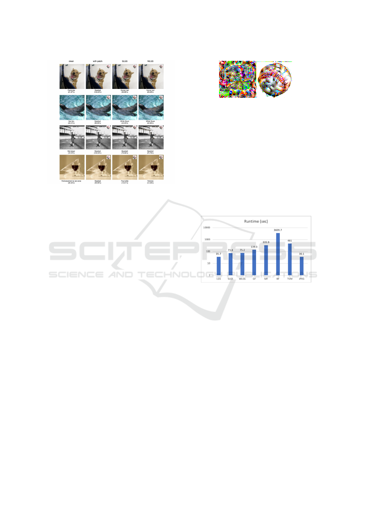
Figure 7: Illustrating failed cases of our methods.

99 percent of the success rate on VGG16. In contrast,

if the attack is not as successful, or if the model is

robust to such attack methods, the effect of our pro-

posed method could be deduced. Our research shows

that Inception-v3 has stronger robustness than other

models, including VGG16, ResNet101 (He et al.,

2016), and GoogLeNet (Szegedy et al., 2015) under

the same attacks. Patch size also affects the perfor-

mance greatly. As we take the “primary” part of the

saliency map in both SLGS and WLGS, we do not

specify how large the proposed region should cover.

Since Adversarial Patch (≈5%) attack covers more

size than LaVAN (up to 2.2%), WLGS has relatively

bad performance with a smaller smooth factor, com-

pared to other methods. This phenomenon leads to

another question: how to choose a suitable smooth

factor? In regards to this, we propose a possible so-

lution to the problem: estimate the patch size using

the local gradient map. Since LGS discussed the cor-

relations between patch attacks and high-frequency

noises, we can calculate the area occupied by the

high-frequency noises and thus adjust the smooth fac-

tor automatically.

Initialization of Patch. The success of Local Gra-

dients Smoothing (LGS) scheme is based on the ob-

servation that attacks introduce concentrated high-

frequency changes at a particular image location.

However, we have found that there is a signiﬁcant

reduction of the high-frequency changes as we ini-

tialize the patch with an image similar to the target

class instead of random noise before starting training.

Our image-initialized version of patches also achieves

a smaller loss than the random-initialized ones under

the same experimental settings. Fig. 8 illustrates base-

ball patches with and without initialization.

Figure 8: Left: baseball patch without initialization. Right:

baseball patch initialized with a similar image.

Computational Cost. The computational burden for

our methods is that we pass the input data into the

deep model two times. At the ﬁrst pass, we feed input

into the classiﬁer and calculate the partial derivative

through backward propagation. After the smoothing

process, we then pass the preprocessed image into the

network for inference. Fig. 9 shows the runtime of

defense methods to process 5000 samples. Follow-

ing the baseline, we use JPEG compression from Pil-

low, Gaussian Filter (GF) and Median Filter (MF),

Bilateral Filter (BF), and Total Variance Minimiza-

tion (TVM) from scikit-learn under python3.6 envi-

ronment.

Figure 9: Comparison of the computational cost processing

5000 images from ImageNet ILSVRC-2012 validation set.

The Histogram is in log scale with actual run time on top of

each bar.

White-box Attack. Our empirical results show that

even when the attacker is aware of our defense mecha-

nism, our proposed methods remain robust. We revise

the optimization problem of LaVAN attack and train

it again, where all the experimental settings remain:

x0 = (1 − m)  x + m  δ

argmax

[M(y = ¯y|T (x0)) − M(y = ˆy|T (x0))]

(13)

where M represents the activations prior to the ﬁnal

softmax layer in the network, ¯y is the target class

and ˆy is the source class, and T is a reactive defense

transformation between LGS, SLGS, and WLGS. As

a result, LaVAN attack can not produce an effec-

tive adversarial patch, as shown in Fig. 10. In-

stead of applying a ﬁlter to the whole (input) im-

age, LGS/SLGS/WLGS methods would eliminate the

salient area beforehand. The area that will be affected

Enhanced Local Gradient Smoothing: Approaches to Attacked-region Identiﬁcation and Defense

261

might change due to the different input data or the ran-

dom position of the patch. This will produce multiple

patterns instead of just one speciﬁc pattern that the

model can easily learn from. The objective function

for LaVAN’s training is formulated as minimizing the

distance between the output and the target class and

also maximizing the distance between the output class

and the source class at the same time. Since it can not

minimize the value of the former unit, it turns out to

maximize the value of the latter and set the patch to

zero.

Figure 10: The success rate of white-box attacks.

5 CONCLUSION REMARKS

5.1 Conclusion

In this work, we propose two revisions of Lo-

cal Gradients Smoothing (LGS) methods, Saliency-

map-based Local Gradients Smoothing (SLGS) and

Weighted Local Gradients Smoothing (WLGS), to de-

tect possible adversarial patches and to remove such

noises accordingly. We attempt to interpret how an

adversarial attack affects from the perspective of the

deep model, i.e., the saliency map, thereby propos-

ing an algorithm integrating the saliency map with

original methods. By locating the adversarial noises

with higher precision, SLGS surpasses the baseline

method by over 1.5% on both clean and attacked data

on VGG16, and WLGS is a more stable solution for

addressing adversarial defense in a wider range of

smooth factors. Since our proposed methods require

two stages, the performance is positively correlated

to the success rate of attacks. As the success of our

method is based on the accurate attacked region de-

tection, it requires the noise to have an impact that is

strong enough for the classiﬁcation model. Hence, in

the cases of stronger attackers (or less robust mod-

els), our proposed algorithms can show more im-

provements. Lastly, we experiment with our proposed

methods on the ImageNet ILSVRC 2012 dataset. The

advantages of this work have been seen by experi-

ments with LaVAN and Adversarial Patch attacks on

both VGG16 and InceptionV3 models.

5.2 Future Work

In this work, we apply the saliency map due to its

simple implementation. Apart from the saliency map,

there are some other works trying to explain or in-

terpret CNN models, including Local Interpretable

Model-agnostic Explanations (LIME) (Ribeiro et al.,

2016), SmoothGrad (Smilkov et al., 2017) and Inte-

grated Gradients (Sundararajan et al., 2017). We ex-

pect the techniques of understanding deep models can

contribute to detection and defense against adversar-

ial attacks.

In the future, we hope that the proposed methods

can be applied with existing applications in computer

vision ﬁelds as a mask before inputs are fed into deep

models. By adding another detecting module that will

give an adversarial score to decide whether there is

an attacker and how powerful it could possibly be,

we expect the system to adjust the smooth factor λ

based on the information automatically. In conclu-

sion, we hope to achieve a real-scene, real-time, and

parameter-free improved resolution.

REFERENCES

Brown, T. B., Man

e, D., Roy, A., Abadi, M., and

Gilmer, J. (2017). Adversarial patch. arXiv preprint

arXiv:1712.09665.

Carlini, N. and Wagner, D. (2017). Towards evaluating the

robustness of neural networks. In 2017 ieee sympo-

sium on security and privacy (sp), pages 39–57. IEEE.

Das, N., Shanbhogue, M., Chen, S.-T., Hohman, F., Li, S.,

Chen, L., Kounavis, M. E., and Chau, D. H. (2018).

Shield: Fast, practical defense and vaccination for

deep learning using jpeg compression. In Proceed-

ings of the 24th ACM SIGKDD International Confer-

ence on Knowledge Discovery & Data Mining, pages

196–204.

Dziugaite, G. K., Ghahramani, Z., and Roy, D. M. (2016). A

study of the effect of jpg compression on adversarial

images. International Society for Bayesian Analysis

(ISBA).

Goodfellow, I. J., Shlens, J., and Szegedy, C. (2015). Ex-

plaining and harnessing adversarial examples. In Ben-

gio, Y. and LeCun, Y., editors, 3rd International Con-

ference on Learning Representations, ICLR.

Hayes, J. (2018). On visible adversarial perturbations &

digital watermarking. In Proceedings of the IEEE

Conference on Computer Vision and Pattern Recog-

nition Workshops, pages 1597–1604.

He, K., Zhang, X., Ren, S., and Sun, J. (2016). Deep resid-

ual learning for image recognition. In Proceedings of

the IEEE conference on computer vision and pattern

recognition, pages 770–778.

Huval, B., Wang, T., Tandon, S., Kiske, J., Song, W.,

Pazhayampallil, J., Andriluka, M., Rajpurkar, P.,

ICAART 2022 - 14th International Conference on Agents and Artiﬁcial Intelligence

262

Migimatsu, T., Cheng-Yue, R., et al. (2015). An em-

pirical evaluation of deep learning on highway driv-

ing. arXiv preprint arXiv:1504.01716.

Karmon, D., Zoran, D., and Goldberg, Y. (2018). Lavan:

Localized and visible adversarial noise. In Interna-

tional Conference on Machine Learning, pages 2507–

2515. PMLR.

Lee, M. and Kolter, Z. (2019). On physical adversarial

patches for object detection. ICML Workshop on Se-

curity and Privacy of Machine Learning.

Li, R., Zhang, H., Yang, P., Huang, C.-C., Zhou, A., Xue,

B., and Zhang, L. (2021). Ensemble defense with data

diversity: Weak correlation implies strong robustness.

arXiv preprint arXiv:2106.02867.

Liu, X., Yang, H., Song, L., Li, H., and Chen, Y. (2019).

Dpatch: Attacking object detectors with adversarial

patches. AAAI Workshop on Artiﬁcial Intelligence

Safety.

Madry, A., Makelov, A., Schmidt, L., Tsipras, D., and

Vladu, A. (2018). Towards deep learning models re-

sistant to adversarial attacks. In International Confer-

ence on Learning Representations.

Mustafa, A., Khan, S., Hayat, M., Goecke, R., Shen, J., and

Shao, L. (2019). Adversarial defense by restricting the

hidden space of deep neural networks. In Proceedings

of the IEEE/CVF International Conference on Com-

puter Vision, pages 3385–3394.

Naseer, M., Khan, S., and Porikli, F. Local gradients

smoothing: Defense against localized adversarial at-

tacks. In 2019 IEEE Winter Conference on Applica-

tions of Computer Vision (WACV), pages 1300–1307.

Papernot, N. and McDaniel, P. (2017). Extending defensive

distillation. arXiv preprint arXiv:1705.05264.

Papernot, N., McDaniel, P., Jha, S., Fredrikson, M., Celik,

Z. B., and Swami, A. (2016a). The limitations of deep

learning in adversarial settings. In 2016 IEEE Euro-

pean symposium on security and privacy (EuroS&P),

pages 372–387. IEEE.

Papernot, N., McDaniel, P., Wu, X., Jha, S., and Swami,

A. (2016b). Distillation as a defense to adversarial

perturbations against deep neural networks. In 2016

IEEE symposium on security and privacy (SP), pages

582–597. IEEE.

Paszke, A., Gross, S., Massa, F., Lerer, A., Bradbury, J.,

Chanan, G., Killeen, T., Lin, Z., Gimelshein, N.,

Antiga, L., et al. (2019). Pytorch: An imperative style,

high-performance deep learning library. Advances

in neural information processing systems, 32:8026–

8037.

Ribeiro, M. T., Singh, S., and Guestrin, C. (2016). ” why

should i trust you?” explaining the predictions of any

classiﬁer. In Proceedings of the 22nd ACM SIGKDD

international conference on knowledge discovery and

data mining, pages 1135–1144.

Russakovsky, O., Deng, J., Su, H., Krause, J., Satheesh, S.,

Ma, S., Huang, Z., Karpathy, A., Khosla, A., Bern-

stein, M., et al. (2015). Imagenet large scale visual

recognition challenge. International journal of com-

puter vision, 115(3):211–252.

Shaham, U., Yamada, Y., and Negahban, S. (2015). Under-

standing adversarial training: Increasing local stabil-

ity of neural nets through robust optimization. arXiv

preprint arXiv:1511.05432.

Shao, R., Shi, Z., Yi, J., Chen, P.-Y., and Hsieh, C.-J.

(2021). Robust text captchas using adversarial exam-

ples. arXiv preprint arXiv:2101.02483.

Shi, C., Xu, X., Ji, S., Bu, K., Chen, J., Beyah, R., and

Wang, T. (2021). Adversarial captchas. IEEE Trans-

actions on Cybernetics.

Simonyan, K., Vedaldi, A., and Zisserman, A. (2013).

Deep inside convolutional networks: Visualising im-

age classiﬁcation models and saliency maps. arXiv

preprint arXiv:1312.6034.

Simonyan, K. and Zisserman, A. (2014). Very deep con-

volutional networks for large-scale image recognition.

arXiv preprint arXiv:1409.1556.

Smilkov, D., Thorat, N., Kim, B., Vi

egas, F., and Watten-

berg, M. (2017). Smoothgrad: removing noise by

adding noise. arXiv preprint arXiv:1706.03825.

Su, J., Vargas, D. V., and Sakurai, K. (2019). One pixel at-

tack for fooling deep neural networks. IEEE Transac-

tions on Evolutionary Computation, 23(5):828–841.

Sundararajan, M., Taly, A., and Yan, Q. (2017). Axiomatic

attribution for deep networks. In International Confer-

ence on Machine Learning, pages 3319–3328. PMLR.

Szegedy, C., Liu, W., Jia, Y., Sermanet, P., Reed, S.,

Anguelov, D., Erhan, D., Vanhoucke, V., and Rabi-

novich, A. (2015). Going deeper with convolutions.

In Proceedings of the IEEE conference on computer

vision and pattern recognition, pages 1–9.

Szegedy, C., Vanhoucke, V., Ioffe, S., Shlens, J., and Wo-

jna, Z. (2016). Rethinking the inception architecture

for computer vision. In Proceedings of the IEEE con-

ference on computer vision and pattern recognition,

pages 2818–2826.

Thys, S., Van Ranst, W., and Goedem

e, T. (2019). Fooling

automated surveillance cameras: adversarial patches

to attack person detection. In Proceedings of the

IEEE/CVF Conference on Computer Vision and Pat-

tern Recognition Workshops, pages 0–0.

Xu, W., Evans, D., and Qi, Y. Feature squeezing: Detecting

adversarial examples in deep neural networks. pages

18–21.

Enhanced Local Gradient Smoothing: Approaches to Attacked-region Identiﬁcation and Defense

263