LIMP: Incremental Multi-agent Path Planning with LPA*

ucahit Alkan Yorgancı

, Fatih Semiz

1,2

and Faruk Polat

Middle East Technical University, Computer Engineering Department, Ankara, Turkey

Aselsan Inc. Defense Systems Technologies Business Sector, Ankara, Turkey

Keywords:

AI, Multi-agent, Pathﬁnding, MAPF, Incremental Planning.

Abstract:

The multi-agent pathﬁnding (MAPF) problem is deﬁned as ﬁnding conﬂict-free paths for more than one agent.

There exist optimal and suboptimal solvers for MAPF, and most of the solvers focus on the MAPF problem

in static environments, but the real world is far away from being static. Motivated by this requirement, in this

paper, we introduce an incremental algorithm to solve MAPF. We focused on discrete-time and discrete space

environments with the unit cost for all edges. We proposed an algorithm called incremental multi-agent path

planning with LPA* (LIMP) and discrete lifelong planning A* (DLPA*) for solving I-MAPF (Incremental

MAPF). LIMP is the combination of two algorithms which are the Conﬂict Based Search D*-lite (CBS-D*-

lite) (Semiz and Polat, 2021) and DLPA*. DLPA* is just a tailored version of the lifelong planning A* (Koenig

et al., 2004) which is an incremental search algorithm for one agent. We have shown that LIMP outperforms

Conﬂict Based Search replanner (CBS-replanner) and CBS-D*-lite (Semiz and Polat, 2021) in terms of speed.

Moreover, in terms of cost, LIMP and CBS-D*-lite perform similarly, and they are close to CBS-replanner.

1 INTRODUCTION

The multi-agent pathﬁnding (MAPF) problem is the

extended version of the classical pathﬁnding problem

for more than one agent. In the MAPF problem, agent

paths should not conﬂict. In other words, agents can

not be in the same location at the same time. Semiz

and Polat (Semiz and Polat, 2021) extended the def-

inition of MAPF and came up with a new variant of

MAPF called incremental multi-agent pathﬁnding (I-

MAPF). In the I-MAPF, the environment can change

during the search; in other words, some paths can be

blocked. This new approach better covers real-world

problems. As the environment is not static in the real

world, environmental changes occur when planning a

path for agents. For example, if we are planning the

routes for cargo delivery trucks, the path costs may

change due to the trafﬁc jams, or some of the paths

might be entirely blocked because of accidents. In

this scenario, classical MAPF algorithms cannot re-

ﬂect these changes efﬁciently and generally plan the

routes from scratch.

Several algorithms are developed to handle the

environmental changes efﬁciently for both MAPF

and classical path planning problems such as CBS-

replanner, CBS-D*-lite and LPA*. More algorithms

are pointed at the related work and the background

sections. Conﬂict Based Search (CBS) is an algo-

rithm that aims to solve the MAPF problem by solv-

ing the conﬂicts in the agent paths by adding con-

straints (Sharon et al., 2015). CBS-replanner is the

extended version of the CBS that replans the paths af-

ter an environmental change occurs. In this paper, we

proposed two algorithms named incremental multi-

agent path planning with LPA* (LIMP) and DLPA*.

DLPA* is a version of a former incremental pathﬁnd-

ing algorithm lifelong planning A* (LPA*). LIMP

combines DLPA* with Conﬂict Based Search D*-lite

(CBS-D*-lite). The intuition behind the DLPA* is

that environmental changes (path blocking) generally

affect only the nodes close to the node that the change

occurred. So, the algorithm only re-expands the nodes

near the change, and if the cost of the node changes,

it re-expands the children of this node.

2 RELATED WORK AND

BACKGROUND

2.1 Incremental Pathﬁnding Algorithms

There are many studies focusing on incremental

single-agent pathﬁnding in the literature. Lumel-

208

Yorgancı, M., Semiz, F. and Polat, F.

LIMP: Incremental Multi-agent Path Planning with LPA.

DOI: 10.5220/0010824400003116

In Proceedings of the 14th International Conference on Agents and Artiﬁcial Intelligence (ICAART 2022) - Volume 1, pages 208-215

ISBN: 978-989-758-547-0; ISSN: 2184-433X

sky and Stepanov (Lumelsky and Stepanov, 1986),

Pinadeh and Snyder (Pirzadeh and Snyder, 1990),

Korf (Korf, 1990) and Zelinsky (Zelinsky, 1992) tried

to use existing information to re-plan the path dy-

namically. Stentz tried to solve the problem by gen-

eralizing the A* algorithm by making it responsive

to environmental changes to use in dynamic envi-

ronments. He developed two algorithms D* (Stentz,

1993) which partially changes the f and g values of

the vertexes when environmental change occurs, and

Focused D*, which is the improved version of the D*

(Stentz, 1995) that focuses on updating the costs to

reduce the number of expanded states. Later, Rama-

lingam came up with an incremental algorithm called

DynamicSWSF-FP (Ramalingam and Reps, 1996) to

solve a similar problem which is a grammar prob-

lem. DynamicSWSF-FP is capable of handling the

arbitrary number of edge insertion, edge deletion, and

cost changes. Koenig (Koenig et al., 2004) combined

A* and DynamicSWSF-FP in Lifelong Planning A*.

He also proposed D*-Lite, which behaves similarly

to D* but algorithmically different. D*-lite is shorter

than the former D*. It includes fewer conditional

branches, which makes it easier to implement and ex-

tend (Koenig and Likhachev, 2002).

Unlike traditional A*, LPA* is capable of han-

dling changes by just expanding the nodes that are

affected by the change. It checks whether the short-

est path from the start to the node is subject to the

edge cost change. The algorithm does that by taking

a minimum of the paths adding edge costs to the par-

ents of the node. If the shortest path is changed, LPA*

updates the node’s g value then marks its children as

their shortest path might also be changed. Child nodes

are pushed to the open list to be expanded later. LPA*

is complete and optimal if the heuristic is consistent

and non-negative.

2.2 MAPF Solvers

MAPF solvers might be optimal, sub-optimal,

reduction-based that reduces the problem to the well-

studied one, centralized or distributed. Solvers may

have different cost functions such as sum-of-costs,

makespan, etc. (Sharon et al., 2015). Standley (Stan-

dley, 2010) proposed an improvement that employs

grouping the agents that do not affect other groups

of agents to reduce the state-space. Later, M* (Wag-

ner and Choset, 2011) which dynamically changes

the branching factor, is released. Sharon et al. de-

veloped Conﬂict Based Search (Sharon et al., 2015),

and Boyarski et al. (Boyarski et al., 2020) provided

an iterative-deepening variant of CBS that uses LPA*

(instead of A*) to ﬁnd low-level paths of the agents.

Conﬂict based search (CBS) is an algorithm that

aims to ﬁnd an optimal solution for the multi-agent

pathﬁnding problem. CBS has two levels: low-level

search and high-level search. The low-level search

is a single agent path planning algorithm that is ca-

pable of satisfying some constraints. In the CBS, a

constraint is formulated as a tuple that contains agent

id, location, time information, which indicates that a

given agent cannot be present in the given location

at the given time. High-level search constructs a tree

called a conﬂict tree to solve the path conﬂicts be-

tween agents. A CBS node consists of constraints and

planned paths. A conﬂict occurs when more than one

agent plans to be at the same position at the same time

step. High-level search expands nodes by adding a

constraint to one of the conﬂicting agents at conﬂict

position. As it expands the nodes in the increasing

cost order, CBS is known to be complete and optimal.

Figure 1: Example run of the CBS with a hypothetical low-

level search. Red lines pair the CBS nodes with the corre-

sponding low-level search result. As can be seen, there is a

conﬂict at (B,3) when time equals 1. CBS expands the root

by constraining the blue and green agents to present at (B,3)

when time is 1 (Semiz and Polat, 2021).

2.3 Dynamic MAPF

There are few studies that solve the dynamic ver-

sion of the MAPF problem. Murano et al. (Murano

et al., 2015) studied multi-agent pathﬁnding in a dy-

namic but predictable environment. Atiq et al. (Atiq

et al., 2020) studied a dynamic version of MAPF

in which existing agents may leave and new agents

may join the environment at different times. Wan et

al. (Wan et al., 2018) worked on a lifelong dynamic

MAPF problem where the dynamism of the problem

comes from adding a new agent to the environment.

Semiz and Polat (Semiz and Polat, 2021) worked on

the I-MAPF problem where nodes in the environment

can become temporarily unavailable. They provided

CBS-replanner and CBS-D*-lite solutions. Unlike

classical CBS, when an environmental change occurs,

CBS-D*-lite tries to use a previously constructed con-

ﬂict tree to get the solution faster.

CBS-D*-lite has three stages of handling environ-

mental changes. After an environmental change oc-

curs, CBS-D*-lite starts with its ﬁrst stage and tries

LIMP: Incremental Multi-agent Path Planning with LPA

209

to ﬁnd a sub-optimal solution that satisﬁes some opti-

mization criterion by performing the low-level search

on the goal node of the previously constructed conﬂict

tree. If it fails to ﬁnd such a solution, it moves to the

second stage, in which it performs a high-level search

on a tree whose root is the previous goal node. If it

fails again, it just simply constructs the conﬂict tree

from scratch with the new environment. CBS-D*-lite

uses D*-lite in the low-level search. The algorithm is

complete but not optimal (Semiz and Polat, 2021).

3 INCREMENTAL MAPF WITH

LPA*

The main problem that we are solving is the I-MAPF,

an extended version of the MAPF problem. The input

of the I-MAPF problem consists of:

• A set of k agents {a

, ··· , a

}

• An undirected unweighted graph G = (V, E)

which represents the environment. In the scope

of this paper we used 4-connected grid world.

• A set of starting vertices {s

, ··· , s

} where s

the starting vertex of a

• A set of goal vertices {g

, ··· , g

} where g

repre-

sents the goal vertex of a

• A set of environmental changes E =

{(v

, ∆

), ··· , (v

, ∆

)} where v

is the

vertex which will be blocked. t

is the time when

the vertex is started to be blocked. Lastly, ∆

the blocking period of the vertex. To sum up, an

agent can not present at v

between t

and t

+ ∆

The output of the I-MAPF problem is set of paths

...P

} where P

is a sequence of vertexes with time

information without conﬂict or block. Formally, P

{(v

, 0), (v

, 1), ··· , (v

, i), (v

i+1

), ··· , (v

, m)}

where v

is the start vertex of a

and v

is the goal

vertex of a

(i.e., v

= s

and v

= g

). Formally, a con-

ﬂict is vertex, time and set of agents tuple c = (v, t, A)

where |A| > 1 ∧ ∀a

∈ A(v, t) ∈ P

. Blocking occurs

when there is a blocked vertex-time tuple in the

path. Formally, (v, t) is blocked if ∃(v

, ∆

) ∈ E

= v ∧ t

< t < t

+ ∆

. Lastly, a vertex cannot be

blocked if there exists an agent.

In the high-level search, LIMP uses CBS-D*-lite

as it is. On the other hand, we have developed a mod-

iﬁed version of LPA* named discrete lifelong plan-

ning A* (DLPA*) for the low-level search of CBS-

D*-lite. The new version is simpler, making it easier

to implement and modify. In MAPF, an agent might

wait or come to the same position at different time-

steps to ﬁnd an optimal solution. Hence, our ver-

sion is working in the discrete time-space domain. In

addition to classical LPA*, our version has the abil-

ity to add constraints beside obstacles. The DLPA*

has four main procedures, which are replan, addCon-

straint, and makeChange, advance.

Algorithm 1: DLPA*.

Require: I-MAPF simulation {Simulation S}

1: changes = S.new environmental changes

2: for change c

in changes do

3: makeChange(c i)

4: replan()

5: advance()

Replan is the main procedure of the LIMP (Algo-

rithm 2). Whenever an agent path is needed to be re-

planned, this procedure is called with the former Open

and Closed lists. States of the LIMP contain x coor-

dinate, y coordinate and time information. The parent

of a state is like the parents of a state in the space do-

main, except the time of the parent is one less than the

time of the child; similarly, the time of a child is one

more than the time of the parent. In this way, wait-

ing action can be handled by only advancing the time.

The getParents and getChildren functions return the

set containing the parents and children, respectively.

These functions also check obstacles and constraints

and exclude the ineligible states.

Algorithm 2: Replan.

Require: Path Planning Instance

{OPEN,CLOSED, Goal}

1: while OPEN.notEmpty() AND getPath() =

NULL do

2: S ← OPEN.popHighestPriority()  S : {x,y,t

}

3: if getParents(S) = { } then

4: CLOSED.delete(S)

5: for each state s

in getChildren(S) do

6: if CLOSED.get(s

) then

7: OPEN.add(s

)

8: else

9: CLOSED.add(S)

10: for each state s

in getChildren(S) do

11: if CLOSED.get(s

) = NULL then

12: OPEN.add(s

)

13: Return getPath()

LIMP maintains two sets in low-level that are

Open and Closed. Open set stores the states that are

subject to a change and should be examined. Closed

set stores the states that have a path from the start

state. The popHighestPriority function returns the

state with the highest priority with respect to the

ICAART 2022 - 14th International Conference on Agents and Artiﬁcial Intelligence

210

heuristic. In this paper, we used Manhattan distance

as a heuristic. The notEmpty function returns true if

the set is not empty, false otherwise. The add function

adds the given state to the given set. Both Open and

Closed sets are behaving like formal sets, not allow-

ing the duplicates.

The procedure takes states from the Open list until

reaching the goal. The goal state is the state that has

the exact coordinates as the goal location. The get-

Path function returns the path performing a backward

search if the goal is found. As after adding a con-

straint or object, the shortest path cannot be shorter

than the previous shortest path; we ﬁrst check whether

a path from the goal node to the start node exists; if

so, we return this path. The getPath function can be

implemented as a constant time operation when there

is no path by maintaining the information about the

goal state is found or not. If the popped state has no

parents, that means the state is unreachable. So, it is

deleted from the Closed list. If a state becomes un-

reachable, that may lead its children to become un-

reachable, so children of the deleted state are pushed

to the open list. If a state becomes reachable, its chil-

dren are also pushed to the Open list to be expanded

further if they are not on the Closed list.

Algorithm 3: addConstraint.

Require: {OPEN, CLOSED, Constraint }

1: CLOSED.delete(Constraint)

2: OPEN.delete(Constraint)

3: for each state s

in getChildren(Constaint) do

4: if CLOSED.get(s

) then

5: OPEN.add(s

)

Adding constraint to the LIMP is relatively simple

(Algorithm 3). The constrained state is deleted from

the closed set and its children are pushed to the open

list as they might be unreachable.

Algorithm 4: makeChange.

Require: {OPEN, CLOSED, Position, t, ∆

} 

Position : { x, y}

1: i← t

2: while i ≤ t + ∆

3: S← Position.x, Position.y, i

4: addConstraint(S) i ← i + 1

As environmental changes cover a time period,

unlike the constraints, all the states having the exact

coordinates with the change and being in the given pe-

riod should be deleted from the closed list, and chil-

dren of them should be pushed to the open set to be

deleted further (See Algorithm 4). Additionally, as

stated in the description, the problem only covers en-

vironmental changes that constrain states; hence ob-

stacle removal is not implemented, but it can be im-

plemented easily by tailoring the makeChange func-

tion.

Algorithm 5: advance.

Require: {OPEN, CLOSED, t }

1: S

← getCurrentState()  P

: { x, y, t}

2: for each state S do

3: if S.t = t and S 6= S

then

4: addConstraint(S)

The advance function simulates one time-step of

advancement. As after time-step (t) being a state

other than the recently realized state becomes impos-

sible, the function adds constraints to these states.

For example, after three advancements, if an agent

is at (2,2,3) it cannot be present (2,1,3), so this state

should be constrained. The getCurrentState function

returns the state which the agent currently is. The ad-

vance function does not change the calculated path;

however, it affects further replannings. Note that, in

implication, we have used a priority queue (priori-

tizing lower time-steps) storing states in OPEN and

CLOSED sets in order not to inspect all states.

3.1 Example Run

In this section we will show an example run of DLPA*

with a simple planning case including a constraint ad-

dition. The obstacle addition is just consecutive con-

straint addition we just only considered a constraint

addition for simplicity.

(a) Map

(b) Initial

Conﬁguration

Space

(d) Times

(e) Initial Paths

Figure 2: Example run.

Consider the environment in Figure 2 (a). In Figure

2 (b), starting coordinates of agents are shown as a

robot ﬁgure, and goal coordinates with a house ﬁg-

ure having the same colour as the agent. Figure 2

searching in the time-space domain, we divided every

coordinate into nine time spaces. All the squares in

the Figure 2 (c) represent a time-space tuple. Every

coordinate has nine states starting from the upper left

corner, as in Figure 2 (d).

The initial run of the LIMP is indifferent to the

classical CBS and the initial run of the DLPA* is in-

different to the A* in three dimensions. After the ini-

tial run, agents compute their paths as in Figure 2

LIMP: Incremental Multi-agent Path Planning with LPA

211

(e). After the initial plannings, the search space of

the purple agent can be seen in Figure 3 (a) (initial

search space). The green states are the states in the

closed set, and the yellow states represent the states

in the Open list. The path of the purple agent can

be easily obtained by performing a backward search

from the state (A,2,2). The path is (C,2,0) → (B,2,1)

→ (A,2,2).

(a) Initial search

space

(b) After adding

constraint

(d) Iteration-2

(e) Iteration-3

(f) Iteration-4

(g) Final

Figure 3: State spaces of the example run.

It can be easily seen that there is a conﬂict at the

state (B,2,1). The high-level search constraints one of

the agents. In the example, we assumed that the pur-

ple agent is constrained from being at (B,2,1). The

addConstraint function deletes the state (B,2,1) from

the Closed list and pushes (A,2,3) to the Open list as

it is in the Closed list and it is a child of (B,2,1). Fig-

ure 3 (b) (search space after adding constraint) rep-

resents the search space of the purple agent after the

addConstraint function is performed. The red square

indicates the constrained state.

The algorithm takes the state (A,2,2) as it has the

highest priority. The state has no parents; in other

words, (A,2,1) is not in the closed list, (B,2,1) is

constrained, and there is an obstacle at both (A,1,1)

and (A,3,1). So, the state (A,2,2) is deleted from the

closed list. None of the children of the state is in the

Closed set, so the algorithm does not add any state

to the Open set. Figure 3 (c) (iteration-1) shows the

search space after the state (A,2,2) is popped and ex-

amined.

At next iteration, (C,2,1) and (B,2,2) have the

highest priorities. Assume that (B,2,2) is chosen. The

algorithm pops it from the Open set. As it has nei-

ther a parent nor a child and it is not in the Closed set,

it is basically deleted from the Open set. Figure 3

(d) (iteration-2) represents the search space after the

iteration.

Then, the algorithm picks the state (C,2,1). It is

added to the Closed set, and its children (B,2,2) and

(C,2,2) are pushed to the Open set. Figure 3 (e)

(iteration-3) shows the search space after this itera-

tion.

After these iterations, states (B,2,2) and (A,2,3)

are popped from the Open set, respectively and their

children are added to the Open set. Figure 3 (f)

(iteration-4) shows the iterations, respectively.

So the new path of the purple agent can be found

easily by performing backward search from (A,2,3).

The resulting path is (C,2,0) → (C,2,1) → (B,2,2) →

(A,2,3). The ﬁnal iteration can be seen at Figure 3 (g)

(ﬁnal iteration). As the computed path of green agent

was (B,1,0) → (B,2,1) → (B,3,2), there is no conﬂict

in the paths so the LIMP terminates returning given

paths.

3.2 Theoretical Analysis

In this section, we will show that DLPA* is optimal.

In addition, both DLPA* and LIMP are complete. The

DLPA* has the same ﬂow as the LPA*. As in the dis-

crete domain with the constant cost, a vertex is either

connected to a vertex, meaning that it has an edge

with this vertex with cost one, or disconnected to a

vertex, meaning that it has an edge with this vertex

with cost inﬁnity. Assigning the cost of an edge to

inﬁnity has the same effect as deleting the edge from

the map.

In the space-time domain, a state can have an exact

g-value (due to the time property) and an exact f value

(due to the coordinates). So, changing the cost of a

state is only possible when a state is deleted or newly

examined. The cost change in the LPA* corresponds

to the state deletion or addition in the DLPA*.

Adding a constraint in the DLPA* corresponds to

setting all the incoming edges to inﬁnity in the LPA*.

Performing environmental change also corresponds to

setting proper edges to inﬁnity.

Although advance function in DLPA* have no

equivalent in LPA*, adding a constraint to all states in

time t except a state s results in the same search tree

with a search rooted at (s,t). So, it does not break the

optimality or completeness of DLPA*.

As all the operations correspond to an operation in

the LPA*, the DLPA* is just a particular instantiation

of the LPA*. That implies the DLPA* is also com-

plete, sound, and optimal as the LPA* given that the

underlying heuristic is consistent. However, if there

exists no solution, the algorithm does not terminate.

The termination condition should be checked before-

hand.

CBS-D*-lite is not optimal; hence the LIMP is

also not optimal but complete.

ICAART 2022 - 14th International Conference on Agents and Artiﬁcial Intelligence

212

4 EXPERIMENTAL STUDY

There are no studies except the CBS-replanner and

CBS-D*-lite for solving the I-MAPF problem (Semiz

and Polat, 2021). Hence, we compared our results

with the CBS-replanner and the CBS-D*-lite. We

run benchmark tests for all of the three algorithms

in 8 conﬁgurations. A conﬁguration consists of a

map, a number of agents, a number of environmental

changes. We also used varying environmental change

frequencies (4,6,8,12 and 24 number of environmen-

tal changes in one time-step) with different minimum

and the maximum manhattan distances between the

agent’s start and the goal location. Maximum distance

is added to the conﬁguration as the distance highly

affects memory usage, and our test environment has

limited memory. We have used four maps which are

named 8x8, cross, den520d and brc202d, given in 4.

As all of the algorithms compute different paths at

the root of the search, we have chosen different envi-

ronmental changes for different algorithms. This ran-

domness may make individual test cases biased. To

make this not affect the experiment results, we tried

to run various test cases so the distribution of the test

case results might give better insights. We have run

12200 test cases in total. As some of the cases do not

have a solution or some of the environmental changes

may lead dramatic increase in the elapsed time, which

will create abnormality, we limited one test run to

elapse at most 300 seconds and discarded the cases

that one of the algorithms is exceeded the limit. In

addition to the above, we also run handcrafted exper-

iments to check the completeness of the LIMP and

optimality of the DLPA*.

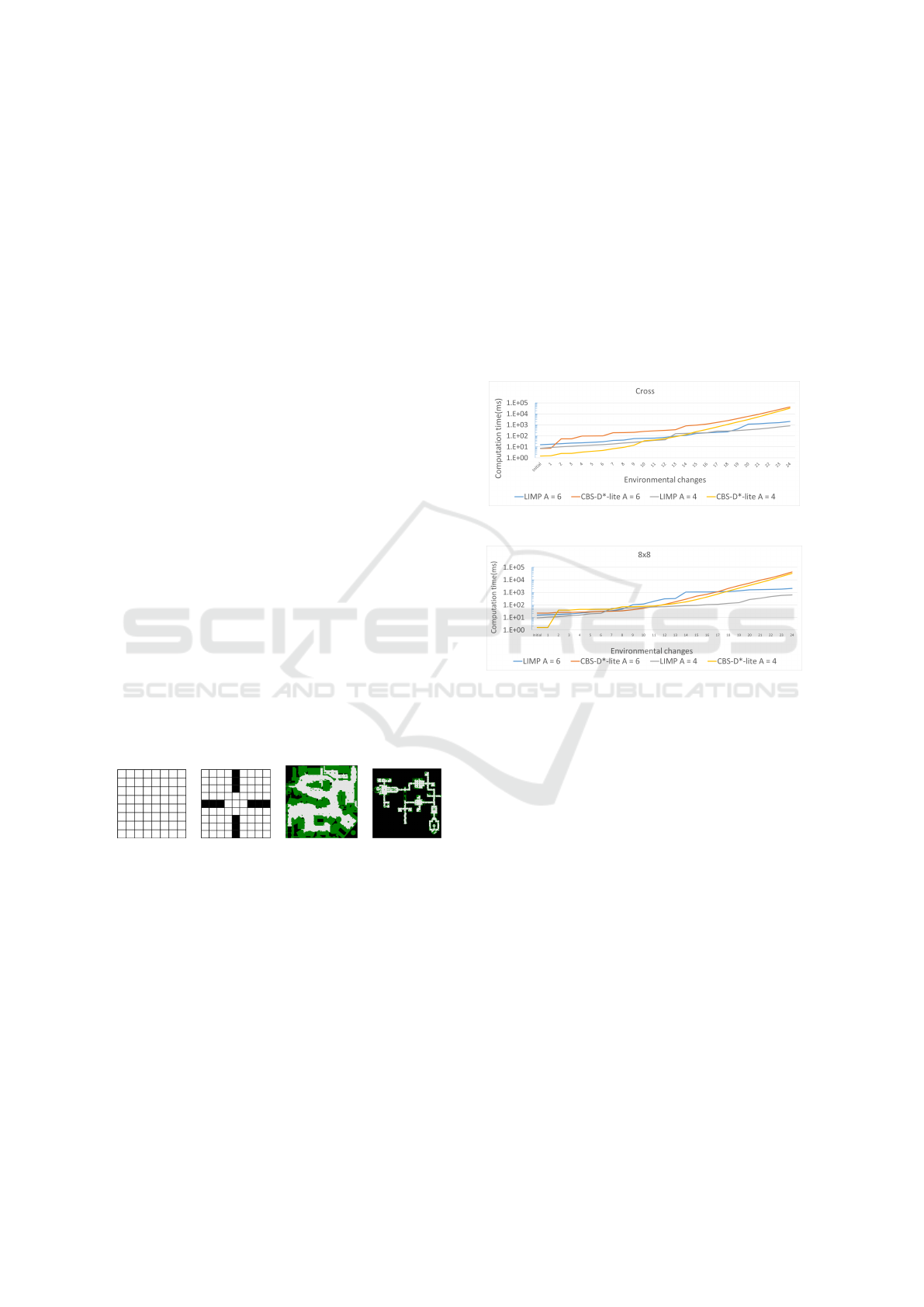
(a) 8x8 (b) Cross (c) Den520d (d) Brc202d

Figure 4: Maps used in the experiments.

We have tested algorithms in 8 conﬁgurations in

the maps 8x8, cross, den520d and brc202d maps.

Den520d and brc202d are the maps taken from

Dragon Age: Origins game. These maps are

commonly used in benchmarking MAPF algorithms

(Sturtevant, 2012). 8x8 environment has an 8x8 grid

without any obstacles. The Cross environment is a

9x9 grid map with a narrow crossing point in the mid-

dle making agents congest more. We have experi-

mented with small maps (8x8 and 9x9) with 4 and

6 agents and larger maps (den520d and brc202d) with

10 and 15 agents. Lastly, we applied 24 environmen-

tal changes to all conﬁgurations.

We have given the results of each conﬁguration in

the following subsections. In the graphs, the x dimen-

sion is the number of environmental changes, the y

dimension is the computation time (ms), and K rep-

resents the number of agents. Note that; results are

reported on a logarithmic scale to ﬁt in the graph.

We have implemented the algorithms using C++. We

have run a benchmark test on a test computer having

AMD Opteron 6376 1.4 MHz core.

4.1 Small Map Scenarios

(a) cross

(b) 8x8

Figure 5: Test results of small map scenarios.

We have run tests on small maps to investigate the per-

formance of LIMP where more congestion happens.

8x8 and cross maps are used for this set of experi-

ments. Since the maps are small, an increase in the

agent count results in high computation times, mak-

ing test cases fail. So we run these cases with a low

number of agents (4 and 6). Figure 5 (a) and (b)

shows the results of the 8x8 map, and Figure 5 (c)

and (d) shows the results of the cross map. For 8x8

map, we have run 1500 and 500 test cases with 4 and 6

agents, respectively. In the cross map (Figure 4b), the

walls separate the map into four sub-parts. The centre

of the map has no obstacles, so agents can move be-

tween the sub-regions, and the crossing region creates

congestion. We have run 2000 and 700 test cases for

the cross map with 4 and 6 agents.

In both maps, LIMP performed worse in the ﬁrst

environmental changes. On the contrary, it out-

performed CBS-D*-lite after several environmental

changes.

LIMP: Incremental Multi-agent Path Planning with LPA

213

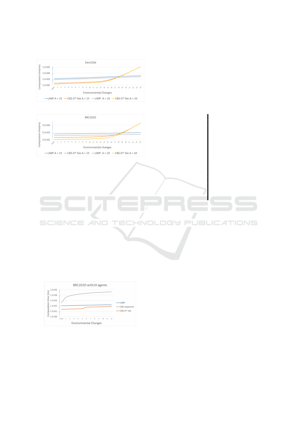
4.2 Large Map Scenarios

(a) Den520d

(b) Brc202d

Figure 6: Test results of large map scenarios.

Den520d and brc202d (Figure 4c,d) maps are used to

test the algorithms, common benchmark maps in the

literature. The number of agents is taken as 10 and

15. We have run 2000 and 1000 tests for 10 and 15

agents for each map, respectively. Additionally, we

have tested LIMP with 20, 25 and 30 agents, which

ended with the same results; however, as eliciting ran-

domness factor requires a high number of test cases,

we did not include these in this paper. Figure 6 a

show the results of the den520d map, and Figure 6b

include the results of the brc202d map.

LIMP, in both maps, performed better than CBS-

D*-lite after the 19th environmental change. As a re-

sult, LIMP is a better option in larger environments

where environmental changes are frequent.

4.3 Comparison with CBS-replanner

Figure 7: Computation time comparison of I-MAPF

solvers.

In this section, we compared computation times of

the CBS-replanner, the CBS-D*-lite and LIMP. Be-

cause of the high computational time of the CBS-

replanner, we did not include it in other conﬁgura-

tions. In addition, we lowered the environmental

change count to 12 and only tested with ten agent con-

ﬁgurations. We have run 1500 tests in the brc202d

map. LIMP and CBS-D*-lite strongly outperformed

CBS-replanner as expected. Figure 7 shows compu-

tation times of the three algorithms tested.

4.4 Comparison of Path Costs

Table 1: Cost analysis of brc202d map with 10 agents.

CBS- CBS-

LIMP D*-lite LIMP D*-lite

0 31.59 31.59 13 32.49 31.93

1 31.65 31.59 14 32.56 31.95

2 31.72 31.65 15 32.62 31.98

3 31.80 31.65 16 32.70 32.01

4 31.86 31.69 17 32.76 32.03

5 31.92 31.73 18 32.82 32.06

6 31.98 31.75 19 32.89 32.07

7 32.06 31.78 20 32.96 32.09

8 32.13 31.80 21 33.04 32.11

9 32.20 31.82 22 33.11 32.14

10 32.27 31.85 23 33.16 32.16

11 32.34 31.87 24 33.24 32.18

12 32.41 31.91

In this section, we compared the total path cost values

of the CBS-D*-lite and LIMP. As CBS-D*-lite has a

decent success rate at total path cost, this comparison

will give us an important overview of the success rate

of LIMP. We took the average total path cost of the

resulting paths of the algorithms after each environ-

mental change for each agent in the brc202d map with

ten agents. As other results were similar, we just pre-

sented one conﬁguration. Table 1 shows the average

path costs of each algorithm. Although CBS-D*-lite

has better total path costs, there is no signiﬁcant dif-

ference between CBS-D*-lite and LIMP. This shows

that we did not deviate from the optimal solution.

5 CONCLUSION AND FUTURE

WORK

The existing MAPF algorithms mainly focus on static

environments; however, the real-life problems are far

away from being static. Recently, an incremental ver-

sion of MAPF was proposed by Semiz, and Polat

(Semiz and Polat, 2021). They also proposed two

algorithms to solve the I-MAPF problem with CBS

called CBS-replanner and CBS-D*-lite. The CBS-

replanner uses A* as a low-level search, and CBS-

D*-lite uses D*-lite in the low-level search.

ICAART 2022 - 14th International Conference on Agents and Artiﬁcial Intelligence

214

In this paper, we proposed two algorithms called

LIMP and DLPA*. LIMP is a combination of the

CBS-D*-lite with our new search algorithm DLPA*,

which is the relaxed version of LPA*. DLPA* is com-

plete and optimal, while LIMP is just complete as it

is built on the top of a sub-optimal I-MAPF solver

called CBS-D*-lite. We have seen that, despite falling

behind in initial calculation, LIMP catches up and

outperforms CBS-D*-lite after several changes, and

it shows that LIMP reacts to environmental changes

more efﬁciently. Although D*-lite ﬁnds slightly lower

path-cost solutions, the differences are at an accept-

able level. Hence, LIMP is a good alternative for

solving the I-MAPF problem, especially when envi-

ronmental changes are frequent.

ACKNOWLEDGEMENTS

This work is partially supported by the Scientiﬁc

and Technological Research Council of Turkey under

Grant No 120E504.

REFERENCES

Atiq, B., Patoglu, V., and Erdem, E. (2020). Dynamic multi-

agent path ﬁnding based on conﬂict resolution using

answer set programming. In Proceedings 36th In-

ternational Conference on Logic Programming (Tech-

nical Communications), ICLP Technical Communi-

cations 2020, (Technical Communications) UNICAL,

Rende (CS), Italy, 18-24th September 2020, volume

325, pages 223–229.

Boyarski, E., Felner, A., Harabor, D., Stuckey, P. J., Cohen,

L., Li, J., and Koenig, S. (2020). Iterative-deepening

conﬂict-based search. In Proceedings of the Twenty-

Ninth International Joint Conference on Artiﬁcial In-

telligence, IJCAI-20, pages 4084–4090. Main track.

Koenig, S. and Likhachev, M. (2002). Dlite. In Eighteenth

National Conference on Artiﬁcial Intelligence, page

476–483, USA. American Association for Artiﬁcial

Intelligence.

Koenig, S., Likhachev, M., and Furcy, D. (2004). Lifelong

planning a*. Artiﬁcial Intelligence, 155(1):93–146.

Korf, R. E. (1990). Real-time heuristic search. Artiﬁcial

Intelligence, 42(2):189–211.

Lumelsky, V. and Stepanov, A. (1986). Dynamic path plan-

ning for a mobile automaton with limited information

on the environment. IEEE Transactions on Automatic

Control, 31(11):1058–1063.

Murano, A., Perelli, G., and Rubin, S. (2015). Multi-agent

path planning in known dynamic environments. In

PRIMA 2015: Principles and Practice of Multi-Agent

Systems, pages 218–231.

Pirzadeh, A. and Snyder, W. (1990). A uniﬁed solution to

coverage and search in explored and unexplored ter-

rains using indirect control. In Proceedings., IEEE In-

ternational Conference on Robotics and Automation,

pages 2113–2119 vol.3.

Ramalingam, G. and Reps, T. (1996). An incremental al-

gorithm for a generalization of the shortest-path prob-

lem. Journal of Algorithms, 21(2):267–305.

Semiz, F. and Polat, F. (2021). Incremental multi-agent

path ﬁnding. Future Generation Computer Systems,

116:220–233.

Sharon, G., Stern, R., Felner, A., and Sturtevant, N. R.

(2015). Conﬂict-based search for optimal multi-agent

pathﬁnding. Artiﬁcial Intelligence, 219:40–66.

Standley, T. (2010). Finding optimal solutions to cooper-

ative pathﬁnding problems. Proceedings of the AAAI

Conference on Artiﬁcial Intelligence, 24(1).

Stentz, A. (1993). Optimal and efﬁcient path planning

for unknown and dynamic environments. INTERNA-

TIONAL JOURNAL OF ROBOTICS AND AUTOMA-

TION, 10:89–100.

Stentz, A. (1995). The focussed d* algorithm for real-

time replanning. In In Proceedings of the Inter-

national Joint Conference on Artiﬁcial Intelligence,

pages 1652–1659.

Sturtevant, N. R. (2012). Benchmarks for grid-based

pathﬁnding. IEEE Transactions on Computational In-

telligence and AI in Games, 4(2):144–148.

Wagner, G. and Choset, H. (2011). M*: A complete

multirobot path planning algorithm with performance

bounds. In 2011 IEEE/RSJ International Conference

on Intelligent Robots and Systems, pages 3260–3267.

Wan, Q., Gu, C., Sun, S., Chen, M., Huang, H., and Jia,

X. (2018). Lifelong multi-agent path ﬁnding in a dy-

namic environment. In 2018 15th International Con-

ference on Control, Automation, Robotics and Vision

(ICARCV), pages 875–882.

Zelinsky, A. (1992). A mobile robot exploration algo-

rithm. IEEE Transactions on Robotics and Automa-

tion, 8(6):707–717.

LIMP: Incremental Multi-agent Path Planning with LPA

215