Automatic Identification of Non-biting Midges (Chironomidae) using

Object Detection and Deep Learning Techniques

Jack Hollister

, Rodrigo Vega

and M. A. Hannan Bin Azhar

School of Psychology and Life Sciences, Canterbury Church University, U.K.

School of Engineering, Technology and Design, Canterbury Christ Church University, U.K.

Keywords: Freshwater Ecology, Computer Vison, Object Detection, Image Classification, Chironomidae, Chironomid,

Faster-RCNN, SSD, Raspberry Pi, TensorFlow.

Abstract: This paper introduces an automated method for the identification of chironomid larvae mounted on

microscope slides in the form of a computer-based identification tool using deep learning techniques. Using

images of chironomid head capsules, a series of object detection models were created to classify three genera.

These models were then used to show how pre-training preparation could improve the final performance. The

model comparisons included two object detection frameworks (Faster-RCNN and SSD frameworks), three

balanced image sets (with and without augmentation) and variations of two hyperparameter values (Learning

Rate and Intersection Over Union). All models were reported using mean average precision or mAP. Multiple

runs of each model configuration were carried out to assess statistical significance of the results. The highest

mAP value achieved was 0.751 by Faster-RCNN. Statistical analysis revealed significant differences in mAP

values between the two frameworks. When experimenting with hyperparameter values, the combination of

learning rates and model architectures showed significant relationships. Although all models produced similar

accuracy results (94.4% - 97.8%), the confidence scores varied widely.

1 INTRODUCTION

By measuring the variation in species and their

abundance, biomonitoring assessments can help to

establish the state of an ecosystem (Costa et al.,

2020). It can inform on the quality of water systems,

substrates, or air, and suggest not only what

organisms are present, but what 'should' be present

(Cao et al., 2018). However, these monitoring

systems rely on the correct identification of the

organisms. The two current solutions to this are visual

identification and molecular-based procedures such

as DNA barcoding, but neither is perfect. Visual

methods are prone to mistakes (Haase et al., 2006),

while using DNA barcoding can become incredibly

expensive and time consuming (Shendure et al.,

2017). Using a deep learning based portable platform,

this paper proposes an automated identification

system that is rapid, accurate, cost-effective and

potentially user-friendly.

https://orcid.org/0000-0003-4915-9840

https://orcid.org/0000-0003-1190-6644

1.1 Freshwater Ecosystems

Freshwater ecosystems can be found on all continents

of the world, but they are most common in North

America, Europe and Asia (Siberia). Only 3% of the

world’s water is fresh water, with majority held

within the polar icecaps (Gerbeaux et al., 2016). A

large portion of living organisms relying on fresh

water as a source of sustenance, and the ecosystems

surrounding these waters provide habitats to a broad

range of species, making it important to maintaining

these systems (Hughes, 2019). There are a range of

fresh waters both natural and manmade such as, but

not limited to, rivers, streams, lakes, marshes, chalk

streams and reservoirs. Despite their importance to

providing sustenance to a large selection of life, and

to supporting the surrounding habitats, freshwater

ecosystems are in danger of degradation due to

anthropogenic interference with the main

contributing factors being pollution, climate change

and habitat transformation (Cao et al., 2018). This

256

Hollister, J., Vega, R. and Azhar, M.

Automatic Identiﬁcation of Non-biting Midges (Chironomidae) using Object Detection and Deep Learning Techniques.

DOI: 10.5220/0010822800003122

In Proceedings of the 11th International Conference on Pattern Recognition Applications and Methods (ICPRAM 2022), pages 256-263

ISBN: 978-989-758-549-4; ISSN: 2184-4313

degradation is having a knock-on effect to the

organisms that depend on these ecosystems. For

instance, the global decrease in macroinvertebrate

populations and the decrease in macroinvertebrate

species diversity is being linked directly to this

anthropogenic interference (Costa et al., 2020),

which, in turn is having a wider knock-on effect to the

ecosystem in which these organisms inhabit (Cao et

al., 2018). To prevent this, ecologists and

conservationists can use biomonitoring techniques to

assess these ecosystems in their current and ongoing

condition. For the biomonitoring of all aquatic

ecosystems, the community structure of benthic

macroinvertebrates can be used and can include the

abundance and presence (or lack of) certain species

(Costa et al. 2020).

Cao et al. (2018) proposed that a lack of expected

benthic macroinvertebrate communities and the

presence of certain ubiquitous species, particularly

those considered pollutant tolerant (i.e., sludge-

worms, Tubifex tubifex), could be used as indicators

to show how the degradation of river water is affected

by municipal waste. This type of approach is

routinely used by researchers and governing bodies

across the globe to assess the quality of water systems

and the surrounding ecosystems. Biggs et al. (2000),

commissioned by the United Kingdom (UK)

Environmental Agency, justified the use of benthic

macroinvertebrates, along with macrophytes and their

presence within different water systems across the

UK, as bioindicators and proposed how the use of

these can be used to assess the water condition of

ponds, lakes and rivers, as well as the condition of the

banks of these water systems. While there is a

selection of species that can contribute to these

assessments (i.e. stone fly nymphs, oligochaetes,

caddisfly larvae), chironomid larvae are considered

ideal candidates for such assessments (Rawal et al.,

2018).

1.2 Chironomids

Chironomids, also known as ‘non-biting midges’ or

‘bloodworms’ (when in their larval stage), are one of

the most abundant and species-rich benthic

macroinvertebrates in freshwater ecosystems

(Nicacio et al., 2015). Chironomids are suggested to

make up 50% of the total benthic macroinvertebrate

population within their respective habitats (Nadjla et

al., 2013). They are found in almost all freshwater

ecosystems including lakes, ponds, swamps, streams

and rivers, and can also be found within isolated

habitats such as tree stumps, and man-made water

ways like flood-prevention drainages. There are an

estimated 600 species found within the United

Kingdom and an estimated 20,000 species worldwide

(Ferrington, 2008). Some species of chironomids can

live in a variety of aquatic systems tolerating a range

of environmental conditions including pH, salinity,

temperature, and sediments, while others require very

specific conditions (Lencioni et al., 2012), and some

can even be found in aquatic systems considered

polluted and inhabitable for most other species

(Luoto, 2011). This has led to the exploration of

chironomids as bioindicators for the general

condition of aquatic ecosystems (Vega et al., 2021),

however, they can also be used for more specific and

streamlined assessments. For instance, Orendt (1999)

created a technical water monitoring method that

provided an acidity assessment for water systems,

where the pH tolerance of 25 species of chironomids

were identified by their presence within several

bodies of water with known pH. Using chironomid

larvae for biomonitoring and paleoclimatic

assessments requires the correct identification to

specific taxonomic levels. However, one of the main

issues with the identification of chironomid larvae is

their minute size. Chironomid larvae are typically

millimetres in length which makes it difficult to

accurately identify them below the taxonomical

classification of family (Chironomidae) without

expert taxonomic knowledge or the means of

molecular-based procedures (Shendure et al., 2017).

1.3 Automated Identification

The use of automatic identification systems is

typically done using computer vison (Azhar et al.,

2012; Ärje et al., 2020), which works with images or

video. These involve techniques such a ‘image

classification’ where a desired subject within an

image can be classified from a set selection of

categories or ‘object detection’, where a desired

subject can be both classified and localised (Rawat et

al., 2017; Huang et al., 2017). The deep learning

techniques, such as Convolutional Neural Network

(CNN), based identifications are growing in

popularity. Bondi et al. (2018) described the

development of an object detection system that uses

techniques from CNNs in order to automatically

detect and identify poachers or high-risk animals in

real-time when used with a video feed. 'PlantSnap' is

another example of integrating deep learning into an

automated identification tool, which can identify and

distinguish over 620,000 different plant species and

their variants from around the world, about 90% of all

described plants (PlantSnap, 2021).

Automatic Identiﬁcation of Non-biting Midges (Chironomidae) using Object Detection and Deep Learning Techniques

257

There are a number of object detection

frameworks, but two of the more popular ones at

present are Single Shot Detection (SSD) and Faster-

Region-based CNNs (Faster-RCNN) (Arcos-Garcia

et al., 2018; Janahiraman et al., 2019; Bose et al.,

2020). With the object detection system built on top

of CNN, a number of possible models can be used,

including SSD_inception, Faster-RCNN_VGG, and

SSD_ResNet (Zhao et al., 2019). SSD is a framework

for detecting objects first described by Liu et al.

(2016). SSD works in a single step, where the CNN

feeds its learned features to the SSD framework and

then places a grid over an image, with each grid space

including an array of possible default locations,

referred to as anchors or bounding boxes. In SSD,

each grid uses the feature maps from the CNN and

assigns the best anchor to predict objects and their

locations within the image.

Ren et al. (2015) introduced Faster-RCNN as a

two-step approach for object detection, which builds

on a CNN to learn features that are then passed to two

separate functions. One is a regional proposal

network that uses a sliding window approach, but

each window has its own set of anchors. These

anchors will use the feature map to detect any

subjects, but only indicate that there is a subject

within the location and does not define a class for the

location. The second function is the one that defines

the class. These types of deep learning systems

require a training period during which images are fed

into the system, causing the system to learn to

recognise the target within a set of images over time.

Several fine-tuning techniques can be applied to

enhance this training process, including adjusting the

hyperparameters and the quality of the data provided

(Probst et al., 2019; Chudzik et al., 2020).

2 METHODOLOGY

An object detection model designed for three distinct

genera of chironomids (Rheotanytarsus, Cricotopus

and Eukiefferiella) was developed in this

investigation. Two different frameworks were used,

Faster-RCNN (FR) and SSD, in which three different

sets of images (dubbed as A, B and C) were used (255

images, 1500 images and 3000 images respectively).

Following the work of Xia et al. (2018), four learning

rate (LR) hyperparameter values (0.1, 0.001, 0.005,

and 0.0005) were chosen for model performance

comparison. With the optimum LR, three intersection

of union threshold (IOU) values were trailed (0.5, 0.6,

0.7). The IOU threshold is the minimum area allowed

between the overlap of an object detection’s

prediction of where an object is to where it is within

an image with a value between 0 – 1 (Bose et al.,

2020).

Chironomid specimens were collected from the

River Stour in Kent, UK using kick sampling. The

head capsules were mounted on microscope slides

and identified to the genus level. These images were

taken with a Raspberry Pi 3b+ module and a

Raspberry Pi camera v2.1, fitted to a Leica DM 500

high powered microscope. A 4X objective lens was

used for all images (40X total magnification). The

microscope has an internal light source, so no

additional light sources were needed. Microscope

slides containing the mounted specimens of

chironomid larvae were placed on the microscope

stage, secured in place by the stage clips, and images

of the slides were taken. For each microscope slide,

three or four chironomid larvae were mounted with

their head capsules and abdominal segments, and

each specimen was placed under a circular cover slip.

The label on the slide followed the standard labelling

system for specimens mounted on microscope slides

(location, site and date system).

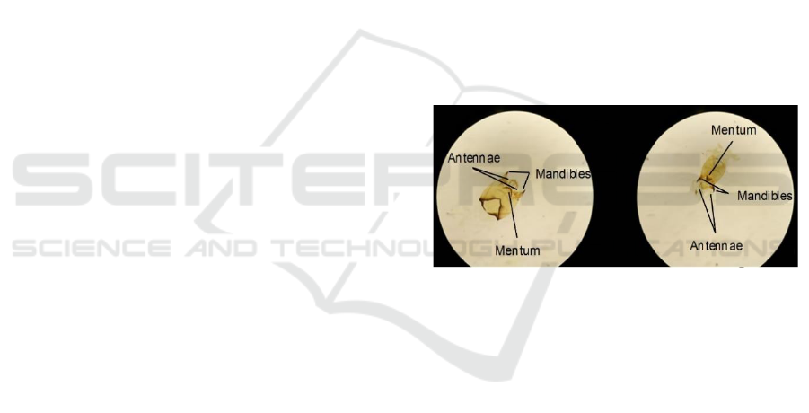
Figure 1: Chironomid larvae head capsules.

Images of two distinct chironomid larvae,

Cricotopus and Eukiefferiella, are shown in Figure 1.

Cricotopus has wide head capsules with thin, curved

mentums, relatively large mandibles and no obvious

antenna. Eukiefferiella has thin head capsules with

dark mandibles and very dark, curved mentums.

Rheotanytarsus has a wide head capsule, mandibles

on the side of their heads, a flat mentum and very

prominent antennae. The mandibles of the three

genera differ in size and shape, so differences in their

shapes and sizes are typically used for morphological

identification and taxonomic classification. The

identified specimens were photographed and the

bounding box labels were applied to the images,

generating a set of co-ordinates for training the object

detection models. An excel reference number was

added so that images could be organized and

referenced easily. Images were separated into their

respective taxonomic group, also known as their

class, at the genus level. There were 863 total images

ICPRAM 2022 - 11th International Conference on Pattern Recognition Applications and Methods

258

taken and used for the three classes (487 Cricotopus,

261 Rheotanytarsus, and 115 Eukiefferiella).

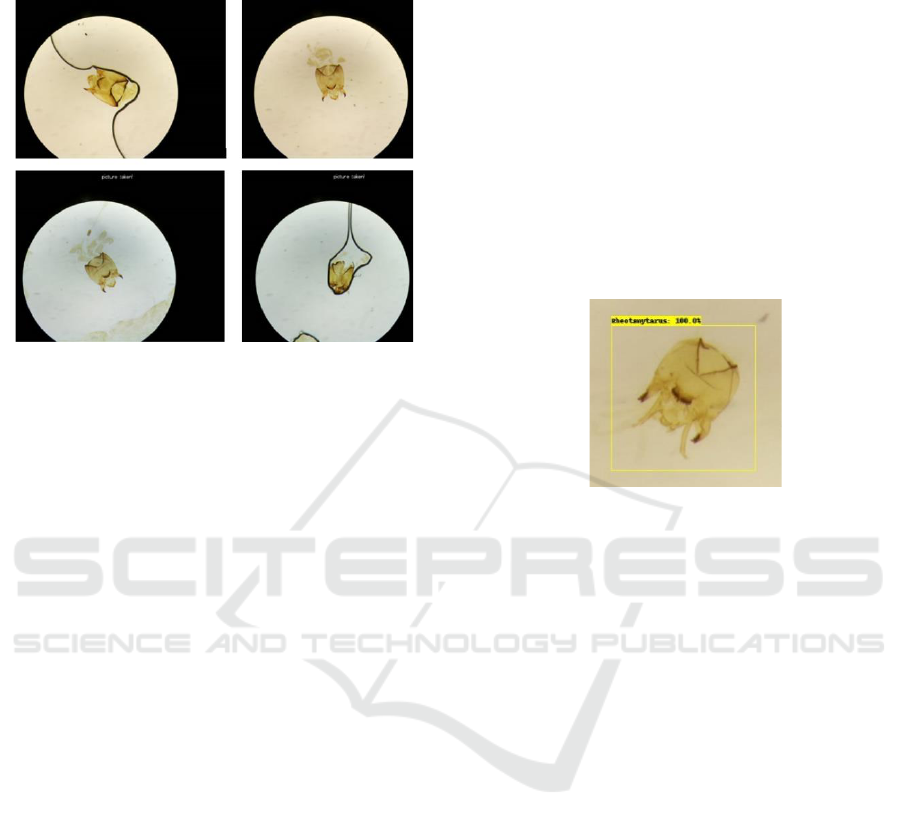
Figure 2: Differences in quality of the images.

Each image contains one chironomid head capsule

of one of three genera, but the quality of the specimen

preparation varies from complete subjects to those

broken apart during mounting procedures or due to

general degradation. Some images contained rear

segments, and some would contain entrails where the

head capsule and rear segments were detached from

each other. Some images also showed wear and

degradation to the slide itself as air and dirt made their

way within the slide. There was also a difference in

the shade of the background on each slide. Figure 2

shows several of the images from the genus

Cricotopus image collection that display differences

in quality, such as the colour of the background, the

completeness of the structure of the head capsule, and

the quality of the slide.

During the training, validation, and testing of the

deep learning models, it was necessary to split the

image sets. To accomplish this, the holdout method

(Yadav et al., 2016) was utilised where a percentage

of the total images was set aside. These images are

taken randomly from the stock of images. In order to

ensure that all models, regardless of image set, could

be evaluated uniformly, 30 images from each class

were set aside for the testing phase. The remaining

images were multiplied to create three image sets (A,

B, and C). In the set A, each class has 85 images.

Thus, to down-sample the majority classes, 85 images

were randomly selected from the original stock within

the Cricotopus and Rheotanytarsus files. In the set B,

each class’s images were up-sampled using

augmentation techniques to create 500 images per

class. For the image set C, images were up-sampled

to 1000 images per class. Several augmentations were

used during the experiments, including rotation to the

left up to 180 degrees, rotation to the right up to 180

degrees, zooming in, zooming out, a horizontal flip,

and a vertical flip. Each image set was split 90:10 for

training and validation respectively.

The training was performed in TensorFlow 1.15,

batch size for each algorithm was 10 and image size

was 300x300. All iterations were run for 5000

epochs. Both object detection frameworks used the

CNN ‘Inception v2’ and the ‘MS COCO’ evaluation

protocols (TensorFlow, 2021). Pretrained models

were downloaded from TensorFlow and used as

transfer learning checkpoints. The mean average

precision or mAP metric was used to evaluate

different object detection models.

Figure 3: Example of a prediction during testing.

Once the models were trained, they were used to

classify specific objects (the chironomid larva head)

from the batch of 90 test images. Figure 3 shows part

of a test image being classified by a model as the

genus Rheotanytarsus, with a confidence score of

100%. A single prediction for each of the test images

was recorded. If there were multiple predictions, only

the prediction with the highest confidence score

would be recorded. Detection thresholds for positive

classification were adjusted to allow all images to be

detected regardless of the confidence value. Using the

confidence scores obtained for all test images, a mean

confidence value was derived for each model.

Additionally, a significance evaluation in the form

of a nested ANOVA (Holmes et al., 2016) was

conducted to examine how different model

configurations were compared, and how image sets

and hyperparameter variations affected the mAP

scores across the trained models. This was then

repeated for the IOU hyperparameter variations while

using the optimum LR for each model configuration

and image set combination. A nested ANOVA can

effectively be broken down into its individual levels

where each could be considered a one-way ANOVA

(Bentler et al., 2010). By following the protocols of a

one-way ANOVA (Doncaster et al., 2007), a

minimum of three repetitions is needed to review the

means of a group for significance, therefore justifying

Automatic Identiﬁcation of Non-biting Midges (Chironomidae) using Object Detection and Deep Learning Techniques

259

that the number of repetitions of each respective

model chosen was enough to meet the requirements.

3 RESULTS

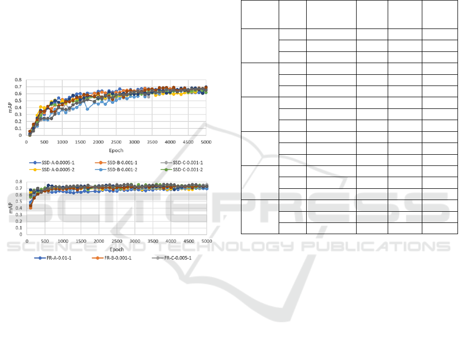
3.1 Results for Varying LR

Figure 4 shows how the mAP values developed over

5000 epochs of training with the SSD and Faster-

RCNN model configurations. All SSD models began

with mAP values near zero and gradually increased.

The FR models, however, produced starting mAP

values of over 0.4, increased rapidly, then levelled off

and maintained an mAP value of approximately 0.7.

Figure 4: The mAP values for varying LR.

Among the SSD models, the configuration SSD-

B-0.005 (Model: SSD, image set B and LR 0.005)

produced the highest mAP value of 0.698. Lowest

mAP value obtained for SSD models was 0.507

produced by the SSD-A-0.01 configuration. For the

FR models, the highest mAP was 0.747 obtained by

the configuration FR-A-0.001. The lowest mAP value

obtained for the FR models was 0.624 produced by

the configuration FR-A-0.0005. Averaging the three

runs for each LR, the mean mAP values for SSD

ranged between 0.579 and 0.678, but for FR ranged

between 0.639 and 0.744.

3.2 LR Accuracy and Confidence

Scores

A high accuracy rate was achieved by all models

(95.6%-97.8%). However, confidence scores varied

widely. The configuration FR-B-0.001 at run 2

achieved an average confidence score of 99.9%,

however, all the FR models had an average

confidence score of over 99%. The SSD models, with

the exception of SSD-A-0.0005 at run 2, all achieved

average confidence scores within the range of 80-

90% (Table 1). The lowest average confidence score

of 80.92% was achieved by the model configuration

SSD-C-0.001 at run 3.

Table 1: LR accuracy and confidence scores.

Model

Config.

Run

Accuracy

(%)

Conf

(%)

Min

Conf

(%)

Max

Conf

(%)

SSD-A-

0.0005

96.7

83.43

100

97.8

91.01

100

97.8

87.64

100

SSD-B-

0.001

95.6

86.84

100

97.8

82.95

100

97.8

89.91

100

SSD-C-

0.001

97.8

86.10

100

97.8

86.78

100

95.6

80.92

100

FR-A-

0.01

95.6

99.04

100

96.7

99.56

100

97.8

99.30

100

FR-B-

0.001

97.8

99.43

100

97.8

99.90

100

97.8

99.80

100

FR-C-

0.005

97.8

99.74

100

97.8

99.18

100

95.6

99.53

100

3.3 Significance Evaluations for LR

Based on the analysis of nested ANOVA, it appears

that the mAP values of the two frameworks were

significant and choice of LR affected the model

configurations, but the selection of image sets did not

affect the mAP values. This produced an R

value of

81.87%. The nested ANOVA was rerun without the

inclusion of the image sets showing significant

differences in mAP values between the two models

and among the LRs within the models (Model:

F=30.920, SS=0.114, p=0.001, LR: F=3.720,

SS=0.022, p=0.003). This produced an R

value of

68.20%. A post-hoc examination (Holmes et al.,

2016) revealed that there was a significant difference

in results between the FR architecture and the

learning rate of 0.0005, and between the SSD

architecture and the learning rate of 0.01 with p-

values <0.05.

3.4 Results for Varying IOUs

Top three model configurations of each framework

(based on the combination of optimum LR values and

ICPRAM 2022 - 11th International Conference on Pattern Recognition Applications and Methods

260

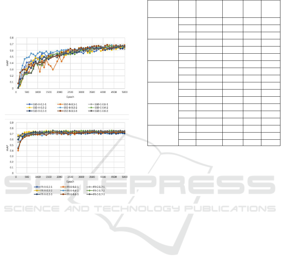
the choice of the image set) were selected to train with

varying IOU settings (0.5, 0.6, 0.7) and each model

was run three times. Averaging the three runs for each

IOU, the mean mAP values for SSD ranged between

0.639 and 0.679, but for the FR models the values

ranged between 0.713 and 0.745.

Figure 5: The mAP values for varying IOUs.

Figure 5 shows how the mAP values developed

during the training over 5000 epochs for the top

performing SSD and FR configurations with varying

IOUs. After 100 epochs, SSD models started with

mAP values near 0 and increased over time, but

remained below 0.7, whereas FR models always

started with values over 0.4, increased rapidly, then

plateaued, and maintained mAP values above 0.7.

3.5 IOU Accuracy and Confidence

Scores

In general, the accuracy scores of all models ranged

from 94.4% to 97.8%, but the confidence scores

differed significantly. The configuration FR-B-0.001-

0.6 (Model: FR, image set B, LR 0.001 and IOU 0.6)

at run 2 achieved the highest average confidence score

of 99.99%, however, all the FR models achieved an

average confidence score above 99% (Table 2). The

configuration SSD-C-0.001-0.6 at run 3 achieved the

lowest average confidence score of 80.92%. The

highest average confidence score for the SSD was

91.98 achieved by SSD-B-0.001-0.5 at run 2.

Table 2: IOU accuracy and confidence scores.

Model

Config

Run

Accuracy

(%)

Conf

(%)

Min

Conf

(%)

Max

Conf

(%)

SSD-A-

0.0005-0.5

96.7

89.42

100

96.7

91.62

100

96.7

81.00

100

SSD-B-

0.001-0.5

95.6

86.37

100

97.8

91.98

100

96.7

91.17

100

SSD-C-

0.001-0.6

97.8

86.10

100

97.8

86.78

100

95.6

80.92

100

FR-A-0.01-

0.5

94.4

99.18

100

96.7

99.46

100

96.7

99.20

100

FR-B- 0.001-

0.6

97.8

99.43

100

97.8

99.99

100

97.8

99.80

100

FR-C-0.005-

0.7

97.8

99.62

100

95.6

99.07

100

97.8

99.54

100

3.6 Significance Evaluations for IOU

The significance of the mAP scores achieved by all

model configurations was evaluated using a nested

ANOVA test by comparing the two frameworks and

how each was affected by the image set and IOUs.

The results show that there were significant

differences between the two frameworks and among

the three image sets: A, B, and C; however, there was

no significant difference among the different IOUs.

This produced an R

of 85.09%. After removing IOU

from the nested ANOVA, the results showed

significant differences in mAP values between the

two models and also among different image sets

within the models. (Model: F=29.79, SS=0.067,

p=0.005, Image Set: F=7.18, SS=0.009, p<0.001).

This produced an R

of 83.48%. The post-hoc test

revealed that there was a significant difference for FR

with image sets A and C and for SSD with image sets

B and C, all with p-values <0.05.

4 CONCLUSIONS

The intention of this study was to create a cost-

effective and fast-working computer-based model

that could act as an identification tool to aid or replace

more traditional methods such as the visual

identification through morphology or by using

molecular methods of identification. The model can

be executed simply with little computer training, and

Automatic Identiﬁcation of Non-biting Midges (Chironomidae) using Object Detection and Deep Learning Techniques

261

can do the identification automatically with high

accuracy (>97%). Using the MS COCO metric

system, the model that produced the highest mAP

value (0.751) was the configuration framework FR

using image-set C, LR 0.005 and IOU 0.7. When

comparing the models, the nested ANOVAs showed

significant differences in mAP values between the

SSD and FR frameworks, as expected from previous

studies (Arcos-Garcia et al., 2018; Janahiraman et al.,

2019), however, any significance between the

remaining factors and variables within the model had

not been explored previously. Almost all of the

models using FR achieved mAP values over 0.7 with

the highest reported value of 0.751, whereas the

models using the SSD framework achieved mAP

values under 0.7 with the highest reported value of

0.698. Interestingly, there was very little difference

between any of the models in terms of accuracy. All

models were able to positively classify the majority

of test images with an accuracy of 94.4% - 97.8%.

Previous studies have shown that there is no

universal LR values (Chudzik et al., 2020),

suggesting that each model and its associated neural

network would require an optimisation of its own LR

value. When experimenting with hyperparameter

values, the combination of learning rates and model

architectures showed significant relationships.

Significant effects were found when the SSD

framework was paired with LR 0.01, and when the

FR framework was paired with LR 0.0005. There was

no significant relationship between the different IOU

values trialled and mAP values. However, there was

a small effect of model performance (1.61%

difference in the strength of the relationship with and

without IOU). Thus, all together, varying the IOU

threshold hyperparameter value could be considered

negligible in the general performance output of the

models.

The deep learning method proposed here utilises

trained object detection models and can classify

images in less than a second. In its present state, the

model using object detection and deep learning

involves chironomids to be collected on a site,

euthanised and their head capsules being placed on

microscope slides. These slides are then viewed

through a microscope lens and images are taken.

Images then need to be transferred to a computer

where they can be examined by the object detection

models which will classify the chironomid head

capsule to one of the three genera. The initial stages

require the use of costly workstations and an expert

to work out the optimum training conditions.

However, once the actual model has been developed,

anyone with access to a computer can use it. When

combined with a camera device, such as an affordable

USB camera, this automatic computer model could be

used to identify chironomid larvae specimens just by

passing them in front of a camera feed rather than

using digital images exclusively. However, it is worth

mentioning that this demonstration only covers a very

small fraction of the chironomid diversity, where only

three genera were detected out of an estimated 200+

genera worldwide and did not distinguish species

taxonomy level, where there are an estimated 20,000+

species worldwide. The use of computer vision

models and, in particular, deep learning techniques

for object detection in ecological sciences are still in

their infancy. This study, however, illustrates how

this technique can be used to rapidly identify

taxonomically challenging organisms. It is envisaged

that future work in object detection will open new

opportunities for biological diversity and

biomonitoring, not only of chironomids but also other

group of freshwater organisms.

REFERENCES

Arcos-García, Á., Álvarez-García, J. and Soria-Morillo, L.

(2018). Evaluation of deep neural networks for traffic

sign detection systems. Neurocomputing, 316, 332-344.

Ärje, J, Melvad, C, Jeppesen, MR, et al. (2020) Automatic

image-based identification and biomass estimation of

invertebrates. Methods in Ecol & Evol.; 11: 922– 931.

https://doi.org/10.1111/2041-210X.13428.

Azhar, M.A.H.B., Hoque, S. and Deravi, F. (2012)

Automatic identification of wildlife using Local Binary

Patterns," IET Conference on Image Processing (IPR

2012), pp. 1-6.

Bentler, P. and Satorra, A. (2010). Testing Model Nesting

and Equivalence. Psychological Methods. 15, 111–123.

Biggs, J., Williams, P., Whitfield, M., Fox, G. and Nicolet,

P. (2000). Biological techniques of still water quality

assessment phase 3: method development. Environment

Agency R & D Technical report E110. Environment

Agency. Bristol. UK.

Bondi, E., Fang, F., Hamilton, M., et al. (2018). Spot

poachers in action: Augmenting conservation drones

with automatic detection in near real time. 32nd AAAI

Conf Artif Intell AAAI, 7741-7746.

Bose, S. and Kumar, V. (2020). Efficient inception V2

based deep convolutional neural network for real-time

hand action recognition. IET Img Proc, 14, 688-696.

Cao, X., Chai, L., Jiang, D., et al. (2018). Loss of

biodiversity alters ecosystem function in freshwater

streams: potential evidence from benthic

macroinvertebrates. Ecosphere, 9, e02445.

Chudzik, P., Mitchell, A., Alkaseem, M., et al. (2020).

Mobile real-time grasshopper detection and data

aggregation framework. Sci Rep, 10, 1150.

ICPRAM 2022 - 11th International Conference on Pattern Recognition Applications and Methods

262

Costa, L., Zalmon, I., Fanini, L., et al. (2020).

Macroinvertebrates as indicators of human disturbances

on sandy beaches: A global review. Ecol Indic, 118,

106764.

Doncaster, C., and Davey, A. (2007). Analysis of variance

and covariance: how to choose and construct models

for the life sciences. Cambridge University Press. UK.

Ferrington, L. (2008). Global diversity of non-biting

midges (Chironomidae; Insecta-Diptera) in freshwater.

Hydrobiologia, 595, 447–455.

Gerbeaux, P., Finlayson, C. and van Dam, A. (2016).

Wetland Classification: Overview. In: Finlayson C. et

al. (eds). The Wetland Book. Springer, Dordrecht, The

Netherlands.

Haase, P., Murray-Bligh, J., Lohse, S, et al. (2006).

Assessing the impact of errors in sorting and identifying

macroinvertebrate samples. Hydrobiologia, 566, 505-

521.

Holmes, D., Moody, P., Dine, D., et al. (2016). Research

methods for the biosciences. Oxford University Press,

Oxford, UK.

Huang, J., Rathod, V., Sun, C., et al. (2017).

Speed/accuracy trade-offs for modern convolutional

object detectors. Proc - 30th IEEE Conf Comput Vis Pat

Rec, CVPR, 296-3305.

Hughes, J. (2019). Freshwater ecology and conservation:

Approaches and techniques. Oxford University Press,

Oxford, UK.

Janahiraman, T. and Subuhan, M. (2019). Traffic light

detection using tensorflow object detection framework.

2019 IEEE 9th Int Conf Syst Eng Technol ICSET 2019

- Proceeding. 108-113.

Lencioni, V., Marziali, L. and Rossaro, B. (2012).

Chironomids as bioindicators of environmental quality

in mountain springs. Freshw Sci, 31, 525-541.

Liu, W., Anguelov, D., Erhan, D., et al. (2016). SSD: Single

Shot MultiBox Detector. Comp Vis, 21-37.

Luoto, T. (2011). The relationship between water quality

and chironomid distribution in Finland - A new

assemblage-based tool for assessments of long-term

nutrient dynamics. Ecol Indic. 11, 255-262.

Nadjla, C., Zineb, B., Lilia, F., et al. (2013). Environmental

factors affecting the distribution of chironomid larvae

of the Seybouse wadi, North-Eastern Algeria. J Limnol.

72, 203214.

Nicacio, G. and Juen, L., (2015). Chironomids as indicators

in freshwater ecosystems: An assessment of the

literature. Insect Conserv Divers. 8, 393-403.

Orendt, C. (1999). Chironomids as bioindicators in

acidified streams: A contribution to the acidity

tolerance of chironomid species with a classification in

sensitivity classes. Int Rev Hydrobiol. 84, 439-449.

PlantSnap (2021). PlantSnap website. Available at

https://www.plantsnap.com. Accessed: 1st November

2021.

Probst, P., Boulesteix, A. and Bischl, B. (2019). Tunability:

Importance of hyperparameters of machine learning

algorithms. J Mach Learn Res. 20, 1-22.

Rawal, D., Verma, H. and Prajapat, G. (2018). Ecological

and economic importance of Chironomids (Diptera).

JETIR, vol. 5.

Rawat W and Wang Z. (2017). Deep Convolutional Neural

Networks for Image Classification: A Comprehensive

Review. Neural Comput. 29, 2352-2449.

Ren, S., He, K., Girshick, R. and Sun, J. (2015). Faster R-

CNN: towards real-time object detection with region

proposal networks. In Proceedings of the 28th

International Conference on Neural Information

Processing Systems - Volume 1 (NIPS'15).

Shendure, J., Balasubramanian, S., Church, G., et al.

(2017). DNA sequencing at 40: Past, present and future.

Nature. 550, 345-353.

Tensorflow (2021), TensorFlow GitHub Model Zoo.

Available at: https://github.com/tensorflow/models/

blob/master/research/object_detection/g3doc/tf1_detec

tion_zoo.md , Accessed: 1st November 2021.

Vega, R, Brooks, S.J., Hockaday, W., et al. (2021).

Diversity of Chironomidae (Diptera) breeding in the

Great Stour, Kent: baseline results from the Westgate

Parks Non-biting Midge Project. J Nat Hist. 55, 11-12.

Xia, D., Chen, P., Wang, B., et al.(2018). Insect Detection

and Classification Based on an Improved

Convolutional Neural Network. Sensors

(Basel).18(12):4169. doi:10.3390/s18124169

Yadav, S., and Shukla, S. (2016). Analysis of k-Fold Cross-

Validation over Hold-Out Validation on Colossal

Datasets for Quality Classification. IACC, 78-83.

Zhao, Z.Q., Zheng, P., Xu, S.T. and Wu, X., (2019). Object

detection with deep learning: A review. IEEE Trans

Neural Netw Learn Syst, 30, 3212-3232.

Automatic Identiﬁcation of Non-biting Midges (Chironomidae) using Object Detection and Deep Learning Techniques

263