Investigation of Capsule Networks Regarding their Potential of

Explainability and Image Rankings

Felizia Quetscher

, Christof Kaufmann

and J

org Frochte

Bochum University of Applied Science, 42579 Heiligenhaus, Germany

Keywords:

Explainability, Capsule Networks, Dynamic Routing, Classiﬁcation, Image Recognition.

Abstract:

Explainable Artiﬁcial Intelligence (AI) is a long-ranged goal, which can be approached from different view-

points. One way is to simplify the complex AI model into an explainable one, another way uses post-

processing to highlight the most important input features for the classiﬁcation. In this work, we focus on

the explanation of image classiﬁcation using capsule networks with dynamic routing. We train a capsule net-

work on the EMNIST letter dataset and examine the model regarding its explanatory potential. We show that

the length of the class speciﬁc vectors (squash vectors) of the capsule network can be interpreted as predicted

probability and it correlates with the agreement between the decoded image and the original image. We use

the predicted probabilities to rank images within one class. By decoding different squash vectors, we visualize

the interpretation of the image as the corresponding classes. Eventually, we create a set of modiﬁed letters

to examine which features contribute to the perception of letters. We conclude that this decoding of squash

vectors provides a quantiﬁable tool towards explainability in AI applications. The explanations are trustworthy

through the relation between the capsule network’s prediction and the corresponding visualization.

1 INTRODUCTION

Through the rise of machine learning applications

the demand for their explainability is increasing. In

the report Guidelines for Trustworthy AI (Ala-Pietil

et al., 2019) the explainability of an AI system is clas-

siﬁed as part of its transparency and it consists of two

elements:

the ability to explain [. . . ] the technical pro-

cesses of an AI system and the related human

decisions

When we use the term explainability, we refer to the

technical part of this deﬁnition. This is further speci-

ﬁed as requirement of an AI system to be understood

[. . . ] by human beings (Ala-Pietil

a et al., 2019). We

interpret this deﬁnition as the reasons that led to a de-

cision of an AI system.

We focus on the classiﬁcation task on images.

Currently, the application of convolutional neural net-

works (CNNs) on this task is the state of the art, see

e. g. He et al. (2016) and Zoph et al. (2018). Despite

the ability of CNNs for image recognition, classiﬁca-

https://orcid.org/0000-0003-1677-5858

https://orcid.org/0000-0002-0191-3341

https://orcid.org/0000-0002-5908-5649

tion and segmentation tasks, their decisions are nei-

ther always self”=explanatory for humans nor always

human-understandable at all.

Multiple approaches provide methods that aim to

explain the results and the vision inside CNNs by iso-

lating or highlighting important areas of the input im-

age. This is done either by the creation of approxi-

mated models (Ribeiro et al., 2016, 2018) or by the

additional calculations based on a trained model (Si-

monyan et al., 2014; Selvaraju et al., 2017). However,

there is no approach yet that leads to a general conclu-

sive solution to explain the vision of CNNs.

Because of the difﬁcult comprehensibility of stan-

dard CNNs, we use an extension to CNNs to improve

the explainability of classiﬁcation tasks. One model

architecture, that seems especially suitable for this

task, is the capsule network (CapsNet) architecture

proposed by Sabour et al. (2017). Their explanatory

potential results from vectors, denoted as capsules,

that potentially store human-understandable features.

In a speciﬁc approach called Dynamic Routing the in-

formation transfer between the capsules is ampliﬁed

or mitigated. During training, the vectors of the last

capsules are masked and then inserted into a decoder

to restore the perceived features of the input image.

After training, the decoder supports explaining the

Quetscher, F., Kaufmann, C. and Frochte, J.

Investigation of Capsule Networks Regarding their Potential of Explainability and Image Rankings.

DOI: 10.5220/0010821600003116

In Proceedings of the 14th International Conference on Agents and Artiﬁcial Intelligence (ICAART 2022) - Volume 3, pages 343-351

ISBN: 978-989-758-547-0; ISSN: 2184-433X

 2022 by SCITEPRESS – Science and Technology Publications, Lda. All rights reser ved

343

perception of the CapsNet.

Subsequently, we use the term CapsNet for the

model that consists of the capsule network itself and

also the decoder. In Sabour et al. (2017), the CapsNet

is trained on the MNIST dataset (Lecun et al., 1998).

It was shown that by modifying the elements inside

the last capsules, features such as stroke thickness,

width or scale change in the digit of the decoded im-

age. Because these features are comparatively human

understandable we examine the potential of CapsNets

to create explanatory results.

We train a CapsNet model on the EMNIST let-

ters (Cohen et al., 2017) dataset. The focus is set on

the ability of the CapsNet to create explanatory image

rankings. The term image ranking refers to the order

of images based on their predicted class probability.

The higher the position of the image in the ranking,

the more it is associated with the considered class.

Firstly, we show that the vectors produced by the

CapsNet are applicable for the creation of image rank-

ings. Secondly, we create and explain the image rank-

ings. The explanation is performed by the visualiza-

tion of those areas that contributed to the prediction

of the correct class. We extend the explanation by vi-

sualizing those features that contributed to the predic-

tion of other classes. Finally, we explore the speciﬁc

characteristics of letters that are displayed in an im-

age.

Overall, the main contributions of our work is the

examination of a CapsNet’s potential and usability to

• create comprehensible image rankings for images

of the same label and

• improve investigation techniques regarding the

explainability.

2 EXPLANATORY APPROACHES

OF CNNS

As mentioned above, there are in fact explanatory ap-

proaches for CNNs. In this chapter, we provide a

brief overview about the properties of three funda-

mental explanatory approaches of CNNs: We cover

the LIME approach (Ribeiro et al., 2016), occlusion

maps (Zeiler and Fergus, 2014), saliency maps (Si-

monyan et al., 2014) and the Grad-CAM algorithm

(Selvaraju et al., 2017).

The LIME (Local Interpretable Model”=Agnostic

Explanations) approach is a general method to ex-

plain single results of an AI model. It is not limited

to any speciﬁc model architecture. The core idea of

the LIME approach is the substitution of a multidi-

mensional non”=human”=understandable model with

an easier interpretable but linear model as approxima-

tion. It is extended to non-linear approximations by

anchors (Ribeiro et al., 2018). Both approaches result

in the examination and isolation of those image areas

that highly impact the class probability. However, the

results of both approaches show that the isolated areas

differ from those features that humans would use for

their perception.

Occlusion maps as ﬁrst proposed in Zeiler and

Fergus (2014) are created by occluding different parts

of the input image and hence this approach is model-

agnostic as well. Rectangles ﬁlled with gray or ran-

dom noise are often used as occluder. By shifting it

through the image and recording the predicted class

probability, it can provide insights which parts of the

image are important for a speciﬁc class. However, a

drawback is that the size of the occluder can inﬂuence

the quality of the map. Also when different objects of

the same or different classes are visible and a softmax

output is used, occluding other objects can decrease

or increase the class probability, respectively, which

might lead to a wrong impression.

The approach to create saliency maps and the

Grad-CAM algorithm are model-speciﬁc and directly

applied to an available trained CNN model. Saliency

maps visualize prominent pixels from a speciﬁed

layer of a CNN by either using guided backpropaga-

tion (Springenberg et al., 2015) or inserting the output

of a layer into the inverted model structure (Zeiler and

Fergus, 2014). Both methods provide a rough orien-

tation for the important features of a class. However,

due to the evaluation of single outputs, the resulting

features are not related to each other and no explana-

tion for the decision-making of the CNN is included.

The Grad-CAM (Gradient-based Class Activation

Map) algorithm (Selvaraju et al., 2017) computes the

gradient of the last feature maps w. r. t. a speciﬁc

class. The mean gradient of a feature map is used

as its weighting, because it describes its importance

for class. The positive values of the weighted av-

erage of the feature maps yields the class activation

map. It highlights areas in the original image that

increased the predicted class probability. Similar as

saliency maps the results of the Grad-CAM algorithm

are reasonable for a rough orientation for the CNN’s

decision. However, they primarily show that CNNs

rely on different features for the classiﬁcation than hu-

mans.

ICAART 2022 - 14th International Conference on Agents and Artiﬁcial Intelligence

344

Primary

Capsule

[28, 28]

Input Image

[20, 20, 256]

Feature Maps 1

[6, 6, 256]

Feature Maps 2

[1152, 8]

Primary Caps

[26, 16]

High-Level Caps

[26]

Class Probs.

Conv. Layer

[256, 9 × 9]

stride: 1

no padding

Conv. Layer

[256, 9 × 9]

stride: 2

no padding

Reshape

dim: 8

Caps Layer

dim: 16

Vector

Length

[26, 16]

Masked Caps

[416]

Flat Array

[512][1024]

[784]

Flat Decoded Image

[28, 28]

Decoded Image

Flatten

Dense

Layer

ReLU

Dense

Layer

ReLU

Dense

Layer

Sigmoid

Reshape

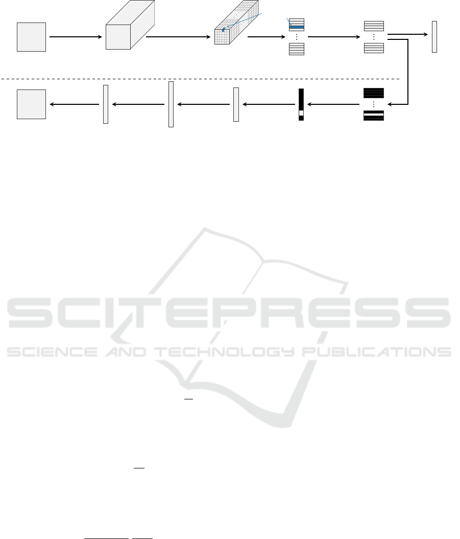
Figure 1: Architecture of a CapsNet with an image input size of 28 × 28 pixels and 26 output classes.

3 ARCHITECTURE OF THE

USED CapsNet

The architecture of our CapsNet is illustrated in Fig-

ure 1. It is based on the architecture proposed by

Sabour et al. (2017). The CapsNet model starts

with two subsequent convolutional layers. We use a

Leaky-ReLU activation function with a leak of a =

0.01 for both convolutional layers. Gagana et al.

(2018) showed that Leaky-ReLU improves the per-

formance compared to plain ReLU. From the output

array of the second convolutional layer (named Fea-

ture Maps 2 in Figure 1) the primary (also: low-level)

capsules are formed by reshaping them. Each primary

capsule consists of a group of n

feature maps (here:

= 8) at a speciﬁc location. The number of values

inside a capsule n

must be a divisor of the number of

feature maps n

(here: n

= 256), such that

is the

number of primary capsules per location (here: 32).

Together with the dimensions [h

, w

, n

] of the fea-

ture maps (here: [6, 6, 256]) it results in the number

of primary capsules (here: N

= 1152).

= h

· w

(1)

Similar to common neurons, capsules also have an

activation function. As in Sabour et al. (2017), we use

the squashing function

g =

||g||

(1 + ||g||

)

||g||

(2)

where g is the vector of a capsule. It squashes the

length of the output vector

g of a capsule between 0

and 1. The resulting length depends non-linearly on g.

The squashing function is performed to both primary

and the subsequent high-level capsules.

The values in a capsule can be interpreted as neu-

rons, since each primary capsule i is fully connected

to each high-level capsule j by a weight matrix W

i j

However, there is no bias vector. The Dynamic Rout-

ing algorithm (Sabour et al., 2017) is executed be-

tween the primary capsules and the high-level cap-

sules. It adds an additional coupling coefﬁcient c

i j

between each primary capsule i and each high-level

capsule j, which stems from a routing logit b

i j

by ap-

plying a softmax across j. The routing logits b

i j

are

initialized with zeros for each forward pass and up-

dated within the routing iterations. Their values re-

sult from the relevance of the prediction of a primary

capsule i to the prediction of a high-level capsule j,

see Procedure 1 in Sabour et al. (2017). As a result,

the connection between both capsules is ampliﬁed or

mitigated.

The number of high-level capsules is equal to the

number of classes. We use the EMNIST letter dataset

(Cohen et al., 2017), which has 26 classes. The num-

ber of values per high-level capsule is arbitrary (here:

16). We refer to the output of a high-level capsule as

high-level squash vector and for the array of all 26

high-level squash vectors as high-level squash array.

On one hand the length of the high-level squash vec-

tors is directly used as predicted class probability. On

the other hand the high-level squash array is passed to

the decoder for the reconstruction of the image.

For the decoder we also use the architecture pro-

posed in Sabour et al. (2017), see the bottom part

of Figure 1. Before the high-level squash array is

inserted into the dense layers of the decoder, it is

masked and ﬂattened. During the training, the mask-

ing is executed for the true class of the input image.

As a result, the values of the high-level squash vec-

tor for the true class stay while the values of all other

high-level squash vectors are set to zero. When we

evaluate the model after training, the masking is done

for one or multiple arbitrary classes, depending on the

purpose of the evaluation.

Investigation of Capsule Networks Regarding their Potential of Explainability and Image Rankings

345

Like in Sabour et al. (2017), we use the margin

loss for the predicted class probabilities L

and the

the mean squared error (MSE) loss for the decoder

. Both loss terms are combined with the weight d:

= L

+ d · L

(3)

This also means, that the decoder is not only respon-

sible to reconstruct the images, rather it provides a

regularization for the CapsNet to learn the class rep-

resentations inside the capsules.

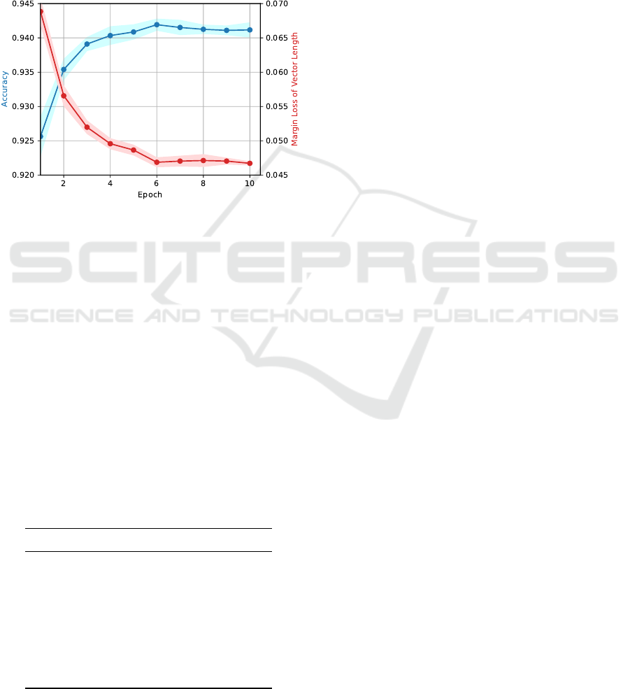
Figure 2: Accuracy and margin loss of the predicted class

probabilities on the test dataset. Solid lines are mean values

and areas are std. dev. of ten runs.

4 TRAINING OF THE CapsNet

The model is trained on the EMNIST letter dataset

(Cohen et al., 2017) that contains 26 classes of hand-

written white letters on a black background. Each

class contains 4800 samples in the training set and

800 in the test set. To train the network we used the

parameters summarized in Table 1.

During the training, the accuracy and the margin

loss L

is recorded for each epoch with a test dataset,

see Figure 2. The loss of class probabilities L

con-

verges faster than the loss of the decoder L

. To avoid

Table 1: Summary of applied parameters to train the Caps-

Net.

Training Parameter Value

Epochs CapsNet (incl. Decoder) 10

Additional Epochs Decoder 20

Batch Size 100

Routing Iterations r 3

High-Level Capsule Dimension 16

Learning Rate 10

−3

Decay Rate per Epoch 0.9

Decoder Loss Weighting d 0.392

overﬁtting the decoder was trained separately for ad-

ditional 20 epochs by providing the masked squash

arrays as input data.

5 PERFORMING IMAGE

RANKINGS WITH A CapsNet

To provide an impression about the appearance of the

high-level squash array, an example for class A is dis-

played in Figure 3. The rows of the squash array

contain the individual squash vectors for class A to

class Z of the EMNIST letters dataset. The ﬁrst row

for class A contains the values with the largest devi-

ation from 0 in both positive and negative direction.

The length of this high-level squash vector, calculated

by the euclidean norm, is indeed 0.95. This value is

signiﬁcantly larger than the lengths of the remaining

high-level squash vectors for the other classes. Con-

sequently, class A is predicted based on this high-level

squash array.

5.1 Validation of the Squash Vector

Length for its Usage in Image

Rankings

Before ranking images by the length of the high-level

squash vector, we conﬁrm that the stored features in a

high-level squash vector are able to represent the im-

age. For that we visualize the stored features by de-

coding the high-level squash array masked for the true

class. Then we measure the quality of the restored

image using the mean structural similarity (SSIM) in-

dex (Wang et al., 2004) between the restored image

and the original image. A scatter plot is created for

all images from the test set relating the SSIM index

with the length of the high-level squash vector for

the true class, see Figure 4. We also compute the

Pearson-Correlation coefﬁcient between the lengths

of the high-level squash vector and the SSIM indices

of the restored images.

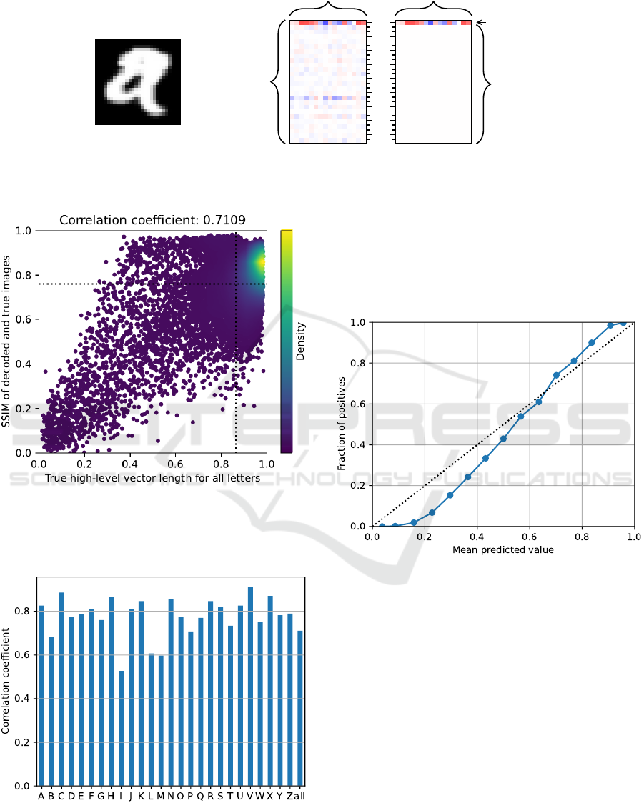
A positive correlation coefﬁcient was found for

each class ranging from 0.53 for class I to 0.91 for

class V. The overview of all correlation values is

shown in Figure 5. This relation supports the assump-

tion that a larger high-level squash vector stores more

features which result in a clearer reconstruction of the

letter. It seems reasonable to evaluate the predicted

class probability of an image by the high-level squash

vector length and to use it for the creation of image

rankings within one class.

Figure 6 shows the calibration plot for all pre-

dicted classes. The calibration curve is monotonically

ICAART 2022 - 14th International Conference on Agents and Artiﬁcial Intelligence

346

unmasked

classes

unmasked

class

masked out

classes

high-level squash vector values

Figure 3: Visualization of a [26 × 16]”=dimensional high-level squash array for the recognition of a sample image of class

A. Left: unmasked squash array, right: squash array masked for class A. A color map from blue to white to red is applied, in

which blue represents negative values, white zero and red positive values.

Figure 4: Correlation of the high-level squash vectors

length for the complete test set with all classes and the cor-

responding mean SSIM index between the original image

and the decoded image from a squash array masked for the

true class. The dotted lines show the mean values.

Figure 5: Correlation coefﬁcients of high-level squash vec-

tor lengths and SSIM indices for each letter and once for all

letters together.

increasing. This strongly supports the application of

the high-level squash vector length for an image rank-

ing, despite that there is a deviation from a perfectly

calibrated curve. Because we do not calibrate the

models, we denote the high-level vector lengths as

predicted probabilities.

Figure 6: Probability calibration plot. The high-level

squash vector length is used as probability. The plot uses

the test dataset and aggregates all classes, where each class

is handled in a one vs. rest manner.

5.2 Creation and Explanation of Image

Rankings

In this section we provide an example for an image

ranking based on high-level squash vectors and their

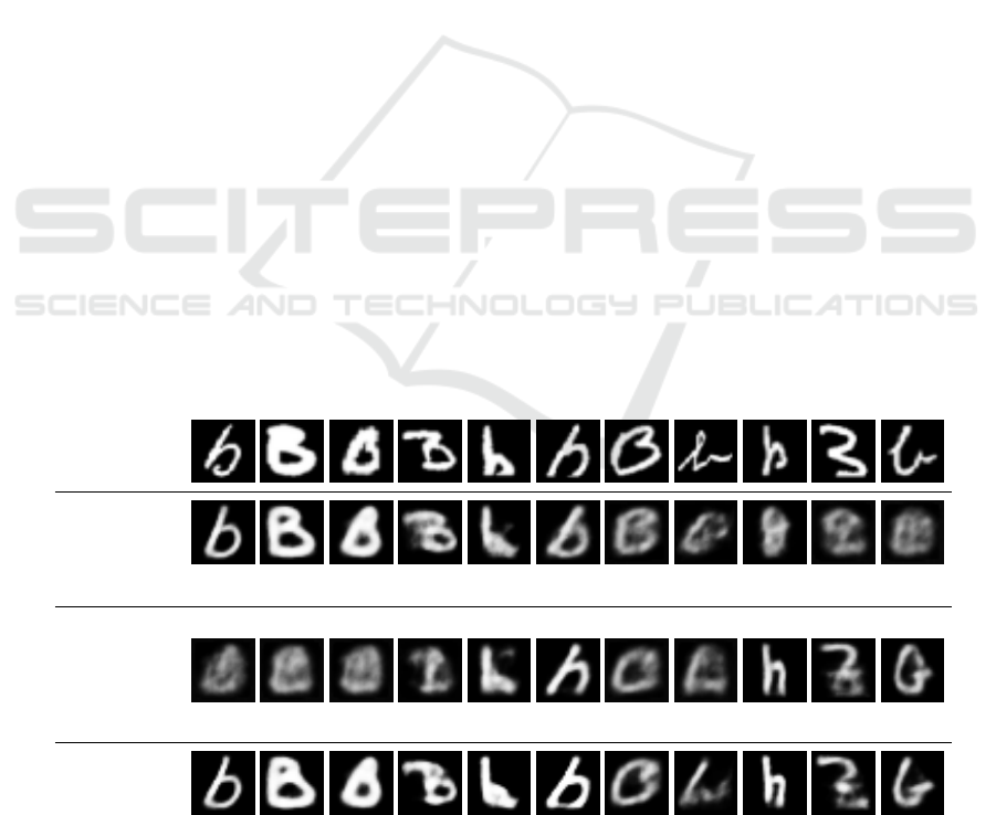
explanation. In Figure 7 we rank eleven test images of

class B with high-level squash vector lengths between

0.95 and 0.11.

One can observe that a small predicted probability

yields a low intensity in the decoded image. Also, the

letters in these reconstructed images appear smoothed

in comparison to the original images. Irregularities,

such as line breaks and additional serifs are recon-

structed only to a small degree. These missing details

Investigation of Capsule Networks Regarding their Potential of Explainability and Image Rankings

347

indicate that the CapsNet tends to learn a generalized

representation of the class. One reason for that might

lay in the rather large [9 × 9] convolutional ﬁlters that

are applied in two convolutional layers.

As discussed in Sabour et al. (2017), when feeding

the decoder with manipulated high-level squash vec-

tors, the characteristics in the decoded image change

in a certain way according to the modiﬁed values.

This provides a way to explainability, but a tedious

one, since the features are different for each class and

might be hard to interpret. We use a different way.

By masking the high-level squash array for different

classes, the decoder reconstructs images of the corre-

sponding classes. This allows to view the image inter-

preted as different classes. This is most interesting for

classes with large predicted probabilities to visualize

which part of the image contributed to the prediction.

The third image row in Figure 7 shows the de-

coded images based on the high-level squash vector

masked for the class with the highest predicted prob-

ability, while ignoring the predicted probability for

the true class B. The quality of these reconstructed

letters depends strongly on the level of the predicted

probability. Above a predicted probability of 0.80, the

decoded letter is recognizable in all instances, while

below 0.80 the letter is recognizable in some cases.

By the decoded images for the true class and for

the class with the remaining largest squash vector we

show how the letters are perceived by the CapsNet.

Their areas cannot be transferred directly to the input

image but rather they indicate why a letter was rated

with a high probability. Good examples are the im-

ages in the sixth and ninth columns in Figure 7. These

might be a small b with a missing part in the bottom

or a small h. The highest predicted probability is at

the class H, but the class B also gets a high probabil-

ity. The decoder together with the masking provides

a method to see how the image can be interpreted as

small b or h. This might also work for occluded image

parts. The restoring of the missing characteristics of

a class also supports the hypothesis that the CapsNet

learns generalized shapes of the classes.

When both high-level squash vectors of one image

have a large difference to each other, the recognition

by the CapsNet is clear. However, the smaller the dif-

ference between the lengths of both high-level squash

vectors, the larger is the ambiguity found in the orig-

inal image. This is often the case for the combination

of two high-level squash vector lengths between 0.30

and 0.80.

The last image row in Figure 7 shows the decoded

image based on a high-level squash array masked for

both classes included above. Through those images

the interaction between the high-level squash vectors

is visualized. The closer the lengths of both high-level

squash vectors, the stronger is their mutual impact on

the dual masked image. The impact is especially high

in the range if the difference between both lengths is

small.

As a result, the certainty for recognized features

correlates with the length of the high-level squash

vector. Through this relation a connection between

the predicted class probability and the explanations is

created. Thereby, the explainability results directly

from the predictions of the CapsNet which leads to

trustworthy results.

To examine which letters are frequently addition-

ally detected in speciﬁc classes, the number of largest

0.95

0.13

0.85

0.24

0.75

0.15

0.65

0.35

0.55

0.42

0.46

0.59

0.36

0.21

0.29

0.23

0.21

0.81

0.18

0.72

0.11

0.74

Original

Masked

Prediction

Class

−

Masked

Prediction

−

Dual Masked

Prediction

Figure 7: Image ranking samples from test dataset for class B based on the high-level squash vector length. The decoded

images, masked for class B, are shown together with the predicted probability of the original sample kv

k in the second row.

The third row shows the decoded images, masked for the class with the largest high-level squash vector that is not B. In the

bottom row the decoded images, masked for both classes is shown.

ICAART 2022 - 14th International Conference on Agents and Artiﬁcial Intelligence

348

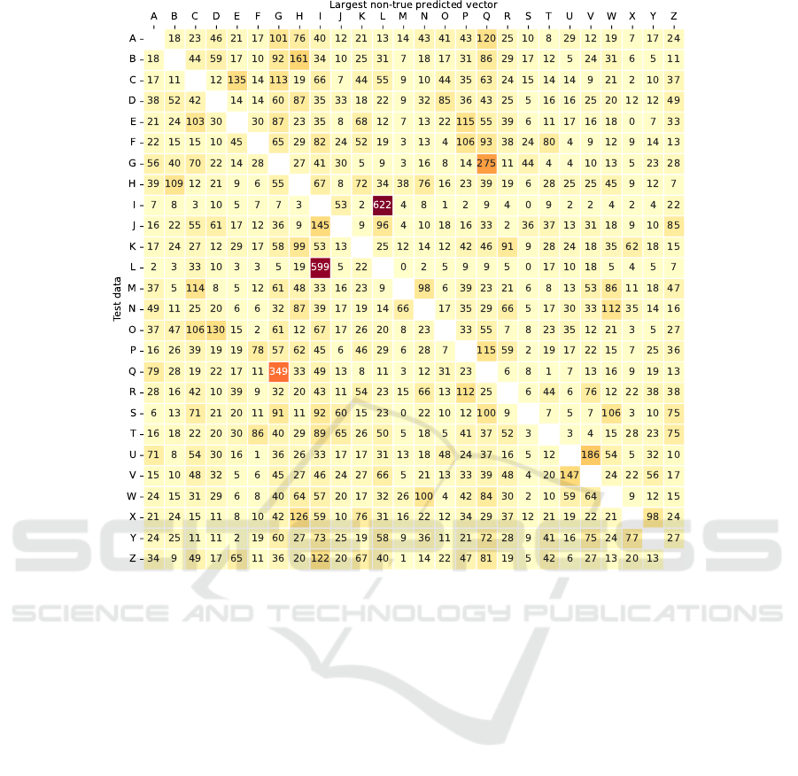
Figure 8: Counts of the highest predicted class probability that is not the true class using the full test dataset.

high-level squash vectors is accumulated for the non-

true class, see Figure 8. We see that the feature of

class L is often found in images of class I (622 times)

and vice versa (599 times). This explains why the

correlation coefﬁcient between the high-level squash

vector length and the SSIM index was low for both

classes. A similar but less distinct phenomenon could

appear at the next high combinations, such as G and Q

(275 and 349 times) as well as U and V (186 and 147

times). The matrix provides an insight to the percep-

tion of the CapsNet because it shows which classes

are found most frequently within other classes.

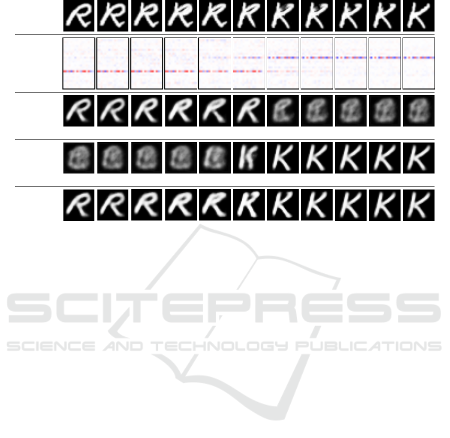
5.3 Exploration of Perceived Features

To explore the characteristics perceived by the Caps-

Net in more detail we create a set of modiﬁed images

that contains the letter pair (R, K) from the test data.

The letter R is gradually transformed to the letter K by

hand, see Figure 9. The images are inserted into the

CapsNet and the resulting high-level squash arrays are

masked for both classes separately. The correspond-

ing decoder outputs and the high-level squash vector

lengths for classes R and K are shown. The lengths

are mostly decreasing for class R while increasing for

class K. As Figure 5 proved, often a larger high-level

squash vector leads to a clearer reconstruction of the

letter. This is conﬁrmed by Figure 9.

The length of the high-level squash vector changes

non-linearly between the samples in Figure 9. There

are one or two images in which the squash vector

length together with the decoded image quality rises

or falls abruptly. According to Figure 6, this behavior

might be a sign for overconﬁdence. The threshold in

the squash vector length could work as a support to

investigate the features that are crucial for the Caps-

Net to detect a class. Apparently in this speciﬁc case,

the top line of the original letter is a decisive factor of

the CapsNet for or against class K. Equally, the con-

nection of the loop for the letter R must have a certain

intensity for the CapsNet to ﬁnd the class R. Several

of the missing features are interpolated, we suspect,

towards generalized letters which maximizes activa-

tion. This assumption is supported by the rise of the

squash vector length from the ﬁfth to the sixth im-

age. We assume, this occurs because the sixth image

resembles one of the generalized letters for class R

more than the ﬁfth image.

Investigation of Capsule Networks Regarding their Potential of Explainability and Image Rankings

349

0.96

0.12

0.94

0.09

0.94

0.07

0.92

0.07

0.71

0.23

0.91

0.48

0.32

0.91

0.14

0.93

0.04

0.95

0.03

0.96

0.05

0.98

Handwritten

Input

High-Level

Squash

Array

R-Masked

Prediction

K -Masked

Prediction

KR-Masked

Prediction

Figure 9: Predictions of the decoder for the image set containing morphed images between the classes K and R.

The explored threshold contributes to the explana-

tory approach with the CapsNet. On this basis, the

characteristics that are important to the recognition

of a class can be extracted. The threshold of two

classes is not necessarily on the same point. This re-

sults in the capability to recognize ambiguous images.

Through the decoding of the squash array masked for

one class it is explainable which characteristics of the

input image were perceived by the CapsNet. Further-

more, the ambiguous letters are also letters that are

ambiguous for the human perception.

6 CONCLUSION AND FUTURE

PROSPECTS

In the introduction we referred to the term explain-

ability as an AI system that is understood [. . . ] by hu-

man beings (Ala-Pietil

a et al., 2019). With the high-

level squash array of the CapsNet together with the

decoder we examined a strong explanatory tool. We

showed that the length of the high-level squash vector

is applicable as predicted class probability and that a

ranking based on its length is reasonable.

The image rankings were explained by decoding

speciﬁc high-level squash vectors. The resulting char-

acteristics showed how the images can be interpreted

as the true class and as another class. Thereby, we

could explain which areas were misrecognized by

the CapsNet. Based on the high-level squash vector

length we could explain the degree of the misinter-

pretation. Finally we showed, based on the transfor-

mation of speciﬁc images that the features used by the

CapsNet are comparable to the human recognition.

In conclusion, the length of squash vector pro-

vides an explainable and quantiﬁable tool for image

classiﬁcation. Its advantage above post-hoc explana-

tory approaches is the connection of the class proba-

bility and the explanation by visualizing the features

of the high-level squash array. Both outputs rely on

the values stored in the high-level squash array result-

ing in a high trustworthiness of the explanations.

ACKNOWLEDGEMENTS

The authors of this work were funded by SUMA e. V.

as well as the federal state of North Rhine-Westphalia

and the European Regional Development Fund FKZ:

ERFE-040021.

REFERENCES

Ala-Pietil

a, P., Bauer, W., Bergmann, U., and Bietlikov

M. (2019). Ethics guidelines for trustworthy AI. EU

Publications.

Cohen, G., Afshar, S., Tapson, J., and van Schaik, A.

(2017). EMNIST: Extending MNIST to handwrit-

ten letters. In 2017 International Joint Conference on

Neural Networks (IJCNN), pages 2921–2926.

Gagana, B., Athri, H. U., and Natarajan, S. (2018). Activa-

tion function optimizations for capsule networks. In

2018 International Conference on Advances in Com-

puting, Communications and Informatics (ICACCI),

pages 1172–1178. IEEE.

ICAART 2022 - 14th International Conference on Agents and Artiﬁcial Intelligence

350

He, K., Zhang, X., Ren, S., and Sun, J. (2016). Deep resid-

ual learning for image recognition. In 2016 IEEE Con-

ference on Computer Vision and Pattern Recognition

(CVPR), pages 770–778.

Lecun, Y., Bottou, L., Bengio, Y., and Haffner, P. (1998).

Gradient-based learning applied to document recogni-

tion. Proceedings of the IEEE, 86(11):2278–2324.

Ribeiro, M. T., Singh, S., and Guestrin, C. (2016). “Why

should I trust you?” Explaining the predictions of any

classiﬁer. In Proceedings of the 22nd ACM SIGKDD

international conference on knowledge discovery and

data mining, pages 1135–1144.

Ribeiro, M. T., Singh, S., and Guestrin, C. (2018). An-

chors: High-Precision Model-Agnostic Explanations.

Proceedings of the AAAI Conference on Artiﬁcial In-

telligence, 32(1).

Sabour, S., Frosst, N., and Hinton, G. E. (2017). Dy-

namic routing between capsules. In Proceedings of

the 31st International Conference on Neural Informa-

tion Processing Systems, NIPS’17, page 3859–3869,

Red Hook, NY, USA. Curran Associates Inc.

Selvaraju, R. R., Cogswell, M., Das, A., Vedantam, R.,

Parikh, D., and Batra, D. (2017). Grad-CAM: Vi-

sual Explanations from Deep Networks via Gradient-

Based Localization. In 2017 IEEE International Con-

ference on Computer Vision (ICCV), pages 618–626.

Simonyan, K., Vedaldi, A., and Zisserman, A. (2014). Deep

Inside Convolutional Networks: Visualising Image

Classiﬁcation Models and Saliency Maps. In Bengio,

Y. and LeCun, Y., editors, 2nd International Confer-

ence on Learning Representations, ICLR 2014, Banff,

AB, Canada, April 14-16, 2014, Workshop Track Pro-

ceedings.

Springenberg, J., Dosovitskiy, A., Brox, T., and Riedmiller,

M. (2015). Striving for simplicity: The all convolu-

tional net. In ICLR (workshop track).

Wang, Z., Bovik, A. C., Sheikh, H. R., and Simoncelli, E. P.

(2004). Image quality assessment: from error visi-

bility to structural similarity. IEEE transactions on

image processing, 13(4):600–612.

Zeiler, M. D. and Fergus, R. (2014). Visualizing and Under-

standing Convolutional Networks. In Fleet, D., Pajdla,

T., Schiele, B., and Tuytelaars, T., editors, Computer

Vision – ECCV 2014, pages 818–833, Cham. Springer

International Publishing.

Zoph, B., Vasudevan, V., Shlens, J., and Le, Q. V. (2018).

Learning transferable architectures for scalable image

recognition. In Proceedings of the IEEE conference on

computer vision and pattern recognition, pages 8697–

8710.

Investigation of Capsule Networks Regarding their Potential of Explainability and Image Rankings

351