
Optimizing Route Planning for Minimising the Non-added-Value
Tasks Times: A Simultaneous Pickup-and-Delivery Problem
Bárbara Romeira
1a
and Ana Moura
1,2 b
1
Department of Economics, Management, Industrial Engineering and Tourism, University of Aveiro, Aveiro, Portugal
2
GOVCOPP – Systems for Decision Support Research Group, University of Aveiro, Portugal
Keywords: Vehicle Routing Problem, Simultaneous Delivery and Pickup, Time Windows, Automotive Industry,
Mathematical Integer Linear Programming Model.
Abstract: The quick-change industrial environment pushes organisations to find new ways to improve efficiency,
flexibility, and responsiveness. To do so, companies must not solely focus on improving the main value chain,
but also the support services that provide for it. To this end, this paper focuses on a route optimization study,
inspired by a real-case problem of the Manufacturing Tool Repair Service, from an automotive company. The
problem consists of a vehicle routing problem with simultaneous delivery and pickup and time windows,
subjected to specific service constraints. To solve it, we propose a Mathematical-Integer Linear Programming
model, which is triggered by real-time data from the shopfloor. The approach was tested, and the results show
an average of 30% improvement compared with the current situation. Additionally, the model was tested
using modified benchmark instances and a time windows sensitivity analysis was performed. Considering the
results obtained, future work regarding the application of a hybrid algorithm is proposed
1 INTRODUCTION
The ever-rising market competitiveness pushes
organisations to find new ways to continuously
improve. As a result, it is not effective for
organisations to simply improve production process.
Rather, they must also improve other services that
support the value chain. In this perspective, the
current work intents to improve the manufacturing
tool pickup and delivery (P&D) service of an
automotive company. This problem is a practical
application of a vehicle routing problem (VRP) with
simultaneous delivery and pickup, and time windows
(VRPSDPTW). When applying time windows (TW)
and simultaneous P&D constraints to the VRP, we
obtained the problem addressed in this paper. Here,
each customer can be, simultaneously, a pickup and a
delivery customer, and the P&D must be done within
pre-defined TW. As it will be presented ahead, the
workers of the Manufacturing Tool Repair (MTR)
service are responsible for picking the used tools from
the production lines, repair them, and, after repair,
deliver them. The absence of real-time information on
a
https://orcid.org/0000-0001-6076-6612
b
https://orcid.org/0000-0003-4687-2747
the number of tools available, forces MTR workers to
constantly leave their workplace, to check the tools’
availability onsite. As a result, time lost travelling
around the shopfloor is significant and the tool repair
activity is constantly delayed. Thus, the present work
intents to optimize this process, eliminating
unnecessary dislocations and minimising the total
travel times, using a Mathematical-Integer Linear
Programming (MILP) model. To do so, it is
considered that: (i) The MTR service uses 2 different
vehicles with distinct capacities; (ii) A production
line is more critical than another, if the time until the
line stops, due to a lack of tools, is smaller. To the
extent of our knowledge, despite the amount of
literature about P&D, the VRPSDPTW is not
commonly considered, although being usual in real-
world situations. Thus, this paper presents the
following contributions:
Application of the VRPSDPTW in a real-
world situation, which considers the demand
and minimal stock requirements at the
customer;
Romeira, B. and Moura, A.
Optimizing Route Planning for Minimising the Non-added-Value Tasks Times: A Simultaneous Pickup-and-Delivery Problem.
DOI: 10.5220/0010821000003117
In Proceedings of the 11th International Conference on Operations Research and Enterprise Systems (ICORES 2022), pages 153-160
ISBN: 978-989-758-548-7; ISSN: 2184-4372
Copyright
c
2022 by SCITEPRESS – Science and Technology Publications, Lda. All rights reserved
153
Real-time route trigger, definition, and
optimization, by connecting the MILP and the
company’s e-Kanban (presented in Romeira et
al. (2021)), which is continuously monitoring
the number of tools to P&D.
This paper is organized as follows: In section 2, a
brief review of other works, related to the
VRPSDPTW is presented. The current problem, the
optimization approach and the data pre-processing
process are described in detail in section 3. In section
4, the MILP model used is shown and the
computational results of our approach are presented
in section 5. Also, additional test results obtained with
benchmark instances and a sensitivity analysis are
presented. A summary and future works are presented
in section 6.
2 RELATED WORKS
In this section a collection of works related to the
VRPSPDTW is offered. Table 1 introduces a
summary of the constraints used in these works, and
Table 2 summarizes the related objective function(s).
In Shahabi-Shahmiri et al. (2021) an hybrid
approach was used to solve the heterogeneous
VRPSPDTW (HVRPSPDTW) with cross-docking
networks, split delivery and perishable products The
authors achieved a 10% reduction in the travel time and
a 29% reduction in the travel costs, when compared to
a previous approach. Zhang et al. (2020) applied two
different approaches to solve the same problem: an
exact and a metaheuristic approach. These were tested
in 15 instances obtained from company data. Their
conclusions show that for larger instances the exact
approach cannot reach the solution in a reasonable
computational time (CPU). Then, the metaheuristic
approach is used to solve those instances and compared
to several state-of-the-art algorithms, showing that it
converges quicker and has a better performance. L. Li
et al. (2019) also solved this problem using a
metaheuristic approach, which, for real-world
instances, obtained solutions within a low CPU time
(81 seconds). In the work of Madankumar and
Rajendran (2019), an exact approach was used and
tested with 24 modified instances given by Solomon
(1987). The results show that it obtained optimal
solutions with better CPU times than the model of
Wang and Chen (2012). Using 8 to 10 of the same
benchmark instances, Gupta et al. (2017) compared
their metaheuristic approach to the best-known results.
For instances C1 and C2, their approach matched the
best-known results, and for R and RC, it obtained
lower travel distances with a small trade-off in the
number of vehicles. Moreover, in real-world instances
it increased flexibility within the company when
compared to the current situation. Besides the
previously referred works, several others may be of
interest. Liu et al. (2021), Zhou et al. (2020), H. Li et
al. (2018) implemented metaheuristic approaches to
solve the VRPSDPTW. Liu et al. (2021) solved the
problem using metaheuristics aiming to minimise the
transportation costs. The approach was tested with
benchmarks instances generated by Wang and Chen
(2012) and the results proved its effectiveness. Having
a multi-objective VRPSDPTW, both Zhou et al. (2020)
and H. Li et al. (2018) applied a metaheuristic
approach. Both approaches outperformed algorithms
proposed by J. Wang et al. (2016) in terms of
convergence and diversity properties. In contrast, Ji
(2019) applied an exact model to minimise the travel
distance. By testing 2 instances of the Solomon (1987)
benchmarks, the author proved that the method is not
suitable for large-size instances. Tang et al. (2021)
proposed a hybrid approach, which found a good
solution in 66% of the benchmark instances (H. F.
Wang & Chen, 2012) and 10 new best-known
solutions. Lastly, Hof and Schneider (2019), using a
hybrid approach, focused on minimising the number of
vehicles, travel distance and TW’s penalties. This
approach, for medium-size instances, reduced the
number of vehicles and the travel distance in 31
instances. For large instances, the best solution had a
16.93% GAP, and used less CPU time than the
approach proposed by Wang et al. (2015).
Table 1: A summary of the VRPSPDTW constraints found in the literature.
Shahabi-Shahmiri
et al. (2021)
Zhang et
al. (2020)
L. Li et al.
(2019)
Madankumar &
Rajendran (2019)
Gupta et al.
(2017)
Our
Work
Vehicles' capacity x x x x x x
Vehicles' type x
Fleet's size x x x
Each customer is visited by only one vehicle x x x x
Time windows (Customers, Workers, etc) x x x x x x
Each customer must be visited exactly once x x x x
Each customer must be assigned to a route x x x x x
Other constraints x x x x x x
ICORES 2022 - 11th International Conference on Operations Research and Enterprise Systems
154
Table 2: A summary of the VRPSPDTW objectives found in the literature.
Shahabi-Shahmiri
et al. (2021)
Zhang et al.
(2020)
L. Li et al.
(2019)
Madankumar &
Rajendran (2019)
Gupta et al.
(2017)
Our
Work
Minimise travel time x x
Minimise travel distance x x
Minimise number of vehicles x
Minimise transportation costs x x x
Minimise waiting times x
Minimise time windows’ penalties x x
Minimise emissions
x
To finish, Table 3 summarizes the approaches
referred throughout this section.
Table 3: A summary of the VRPSPDTW approaches found
in the literature.
Paper Exact
Meta-
heuristic
Hybrid
Liu et al.(2021) x
Shahabi-Shahmiri et al.
(2021)
x
Tang et al. (2021) x
Zhang et al. (2020) x x
Zhou et al. (2020) x
Hof & Schneider (2019) x
Ji (2019) x
L. Li et al. (2019) x
Madankumar & Rajendran
(2019)
x
H. Li et al. (2018) x
Gupta et al. (2017) x
Our Work x
3 CASE STUDY
3.1 Current MTR Service Description
The MTR support service is responsible for the repair
and calibration of the tools used in the company’s
machines. As these tools have limited lifespans,
which are related to the number of parts produced, the
MTR workers pick the used tools from the production
lines, and deliver, new or repaired ones. Currently,
the MTR service team performs the following tasks:
(i) Repair and calibration of tools (Value-added
activity); (ii) Pick used tools from the production
lines; (iii) Deliver repaired, or new, tools to the
production lines. Since no production line must ever
stop for lack of tools, and there is no real-time
information on their availability to be collected, the
MTR workers are forced to go onsite and check the
stocks. This is a waste of time and productivity. Thus,
the P&D activities must be minimised. Currently, to
go to production, the workers follow 3 different
standardized routes (A, B and C – Figure 1). This
process takes an average of 18, 15 and 8 minutes,
respectively. Presently, each route is done at least 2
times per shift. However, sometimes there is an
average of 6 additional trips per shift. The P&D is
performed using one of 2 different vehicles: an
automatic and a manual vehicle. The first has a higher
average speed and a capacity of 150 tools, while the
other a capacity of 90 tools.
3.2 Optimization of the MTR Service
The company’s e-Kanban system, developed in
Romeira et al. (2021), gathers real-time data along the
company’s internal value chain. To this system, it was
added a Manufacturing Tool Stock menu that allows
us to know, in real-time, which tools are available in
each P&D point (the production lines, and from now
on called customers), and how many are available in
the MTR service to be delivered. During, a
production shift, these data is continuously processed,
and a route is triggered when: (i) There are enough
tools available to create a P&D route; (ii) The tools’
stock is below the defined minimum stock values.
This pre-processing gives us the customers to be
visited and the tools to be picked and delivered. Then,
this information, together with all the considerations
related to the vehicles (average speeds and capacities)
and the priority levels of each customer, are used to
compute the routes. The VRPSDPTW is solved using
a MILP model, where the main objective is to
minimise the total travel time for each vehicle,
considering the following general constraints:
Each customer is visited exactly once per route;
MTR service and customers’ TW (these
indicate the priority level);
Vehicles’ capacities.
Figure 2, sums up the process to obtain the inputs
for the MILP model and shows the given outputs. As
can be seen, the e-Kanban is continuously analysing
Optimizing Route Planning for Minimising the Non-added-Value Tasks Times: A Simultaneous Pickup-and-Delivery Problem
155
the tools onsite, and the tools available for delivery in
the MTR service. Also, it is considered that:
All tools have similar dimensions;
The automatic vehicle only serves Route B,
while the manual serves Route A and C;
The vehicles have different average speeds and
service times (the automatic vehicle has a
higher service time);
There are no circulation restrictions;
When a customer has a higher priority (defined
by the stock level), it must be served first;
Every time a route alert is triggered, the MILP
is called to compute a new route.
Data Pre-processing Process. The data pre-
processing process is performed according to the
flowchart in Figure 2, using the data retrieved by the
e-Kanban regarding the tools’ availability in the
customers and in the MTR service. A new route is
created when the stock in a customer is below the
minimal stock level or, when the number of tools
available for P&D is sufficient to make a distribution.
For the first, whenever the minimal stock level is
reached a trip alert is created, because the related
customer is now considered a priority customer.
Then, the decision process is performed according to
the Figure 2 flowchart. Note that, before the MILP is
called, the Availability of tools for P&D procedure
must be performed. This verifies the existence of non-
priority tools to be delivered and picked from these
priority customers, with the aim of using the vehicle’s
full capacity. So, if the vehicle’s capacity is not
achieved with the priority tools, then for the same
priority customers, the algorithm tries to load the
vehicle with tools with the lowest stock level, re-
stocking the customer and/or tools to pick. For the
second option, when there are no tools below the
minimal stock, another procedure is called: Tools for
P&D. Here, it is verified if there are customers with
pickup stock above a pre-determined level, and for
those, the availability of tools to deliver is checked.
4 MILP MODEL
The VRPSDPTW is defined on a direct graph
𝐺𝐶,𝐴) , where the depot and customers are
represented by a set of nodes and with different
geographical location. The set of nodes and the set of
edges in G are represented as 𝐶1,…,𝑐 and 𝐴
𝑖,𝑗):𝑖,𝑗 ∈ 𝐶,𝑖 𝑗 , respectively. The length of
each arc is given by 𝑡
, which is the time needed to
travel from customer 𝑖 to 𝑗. Also, each customer has
a P&D demand, represented by 𝑝
and 𝑑
,
respectively. To deliver the required demand, a set of
vehicles 𝑉0,…,𝑣 is available. Two vehicles are
available, each with capacity 𝑄
,k ∈V. Each
customer
𝑖∈𝐶 must be visited within a predefined
time window 𝑎
,𝑏
], and has a predefined service
time 𝑠𝑡
. Furthermore, the depot node (MTR service)
also has a time window, 𝑎
,𝑏
], which defines the
total time available to execute the P&D requirements
in each shift. To meet the TW, the decision variable
𝑠
defines the arrival time of vehicle k ∈ V to
customer 𝑖 and to the depot. Another decision
variable used is 𝑥
that takes value 1 if arc 𝑖,𝑗) is
traversed by vehicle 𝑘∈𝑉, and zero otherwise.
Considering the nature of the problem, the following
integer variables are also considered:
Figure 1: Route creation process and its outputs.
ICORES 2022 - 11th International Conference on Operations Research and Enterprise Systems
156
𝑙
, gives the total amount of load after vehicle
𝑘 visits customer 𝑖;
𝑙𝑑
, gives the amount of load that remains to
be delivered, by vehicle 𝑘, to customer 𝑖 and to
all the following customers.
𝑙𝑝
, gives the amount of load that must be
picked-up after vehicle 𝑘 visits customer 𝑖.
Taking into consideration the above data and decision
variables, a MILP vehicle-flow model was
developed:
Min t
x
)
(1
)
The objective (equation 1) is to minimise the total
travel time and is subjected to the following
constraints:
x
ij
k
c
i=1, i≠j
=1, ∀ j≠1∈C
v
k=1
(2)
x
ij
k
c
j=1, i≠j
=1, ∀ i≠1∈C
v
k=1
(3)
x
ih
k
c
i=1, i≠h
- x
hj
k
c
j=1,j≠h
=0, ∀ k∈V, ∀ h∈C
(4)
x
1j
k
c
j=1
≤1, ∀ k∈V
(5)
x
i1
k
c
i=1
≤1, ∀ k∈V
(6)
s
i
k
+st
+t
ij
-M
T
1-x
ij
k
≤s
j
k
, ∀ k∈V, ∀ i≠j∈C
(7)
a
i
≤ s
i
k
≤ b
i
, ∀k∈V, ∀ i∈C
(8)
ld
i
k
≥ ld
j
k
+d
i
-M
1
(1-x
ij
k
), ∀ k∈V, ∀i,j≠1∈C
(9)
l
j
k
≥ ld
j
k
+d
j
+p
j
, ∀ k∈V, ∀j≠1∈C
(10)
l
j
k
≥ l
k
+d
j
p
j
-M
2
(1-x
ij
k
), ∀ k∈V, ∀i≠1,j≠1∈C
(11)
d
i
≤ ld
i
k
≤ Q
k
, ∀k∈V, ∀ i∈C
(12
)
p
i
≤ l
i
k
≤ Q
k
, ∀k∈V, ∀ i≠1∈C
(13
)
lp
j
k
≥ lp
i
k
+p
j
-M
3
(1-x
ij
k
), ∀ k∈V, ∀j,i≠1∈C
(14
)
p
i
≤ lp
i
k
≤ Q
k
, ∀k∈V, ∀ i∈C
(15
)
l
i
k
= lp
i
k
+ ld
i
k
-d
i
, ∀k∈V, ∀ i≠1∈C
(16
)
x
ij
k
∈
0,1
;s
i
k
0;l
i
k
,ld
i
k
lp
i
k
0 and integer
(17
)
Constraints (2) and (3) ensure that each customer
is visited exactly once and by only one vehicle.
Constraint (4) guarantees the flow conservation,
which means that if vehicle k arrives at customer i, it
must also leave customer i. Both (5) and (6) ensure
that each vehicle starts and ends its route in the depot.
Inequalities (7) and (8) are related to the TW
constraints. The first specifies the vehicle arrival time
to a customer and the second guarantees that the
vehicle arrives within the related TW. With constraint
(9), the delivery quantity to be loaded at the depot is
specified. Additionally (7) and (9) force an order for
the vehicles visiting the routes, which ensures that no
sub-tours without the depot are generated.
Inequalities (10) and (11) indicate the amount of load
in the vehicles after visiting the first customer and the
other customers in the route, respectively. Constraints
(12) and (13) guarantee that the vehicle capacity is not
exceeded. For more information on the pickup
loadings, 3 more constraints were added. With
inequality (14) the pickup quantity that must be
unloaded in the depot is determined. Constraint (15)
guarantees that the vehicles capacity is not violated,
and constraint (16) correlates the load variables to
each other. Constraint (17) defines the variable’s
domains. Constraints (7), (9), (11) and (14) are
disjunctive constraints that are linearized by using
large multipliers (‘‘big-M values’’). To create valid
inequalities, one set 𝑀𝑇 𝑠
and 𝑀1 𝑀2
𝑀3 𝑚𝑎𝑥𝑄
.
Figure 2: Data pre-processing process.
Optimizing Route Planning for Minimising the Non-added-Value Tasks Times: A Simultaneous Pickup-and-Delivery Problem
157
5 COMPUTATIONAL RESULTS
The model was tested with 10 types of instances from
normal demand requirements and 3 types of instances
with high demand quantities for each type of vehicle
(the worst-case scenario). Thus, in total we analysed
26 instances, 13 for the manual vehicle and other 13
for the automatic vehicle. Each problem instance is
defined by the quantity to P&D to each customer. The
vehicles capacity is given in number of tools, and for
the manual vehicle is equal to 90 and equal 150 for
the automatic. Also, the customer’s location was
obtained from the company’s layout (presented in
Figure 1) and the travel arcs times were calculated
according to each vehicles’ average speed. For each
customer the service times (𝑠𝑡
) and time windows
([𝑎
,
𝑏
]) are defined according to real data. Note that,
the TW are dynamic, based upon the customers’
priority in the route creation moment. Based on this,
the customer with highest priority has earlier and
tighter TW than the others.
Results. The model presented was implemented
using the CPLEX Studio IDE 20.1.0, and the
experiments were run on an Intel (R) CORE(TM) i7-
10750H CPU 2,60GHz with 16Gb of memory.
Table 4 shows the results obtained for the manual
vehicle and Table 5 for the automatic vehicle. In the
tables’ second column, the number of routes that the
vehicle must make (Trips) is presented. This means,
the number of times that the vehicle must leave and
return to the depot to fulfil the demand requirements.
The other columns of the table present the objective
function value (OF) – time needed to perform the
route in minutes, and the CPU time in seconds.
The last column presents the GAP (in %), given
by CPLEX, that is the tolerance on the GAP between
the best integer solution and the best node remaining
(best bound). For the manual vehicle, the results show
that the optimal solution is achieved for 8 of the 13
instances. For the remaining instances the obtained
GAP is in average 5%, except for test instance 8,
where the GAP is 23%. The solutions were obtained
within a low CPU time (average 0.21 seconds). Also,
the number of trips needed to fulfil the customers’
Table 4: MILP results for the manual vehicle.
Instance Trips OF (min) CPU (s) GAP (%)
1 2 9.22 0.17 0
2 2 9.22 0.17 0
3 2 9.22 0.22 5.83
4 2 9.22 0.17 5.04
5 2 9.22 0.09 0
6 2 9.22 0.82 5.1
7 2 9.22 0.13 0
8 2 9.22 0.17 23.03
9 2 9.22 0.16 0
10 2 9.22 0.09 0
11 4 17.77 0.13 0
12 4 15 0.23 4.82
13 4 17.77 0.14 0
demand is 2, except for the last 3 instances (worst-
case scenario instances). These are the ones which
have a high number of P&D demands, which, in some
customers equals the vehicles’ capacity. For the
instances with higher demand values, 2 optimal
solutions were obtained within, approximately, 0.14
seconds. For the automatic vehicle, the model only
reaches the optimum to 3 solutions out of 13.
Although the results obtained have an average GAP
of 9.6%, they were obtained within good CPU time
(17.8 seconds). When it comes to the high demand
instances, the CPU time required is much higher than
the average for other instances, especially for the 11
th
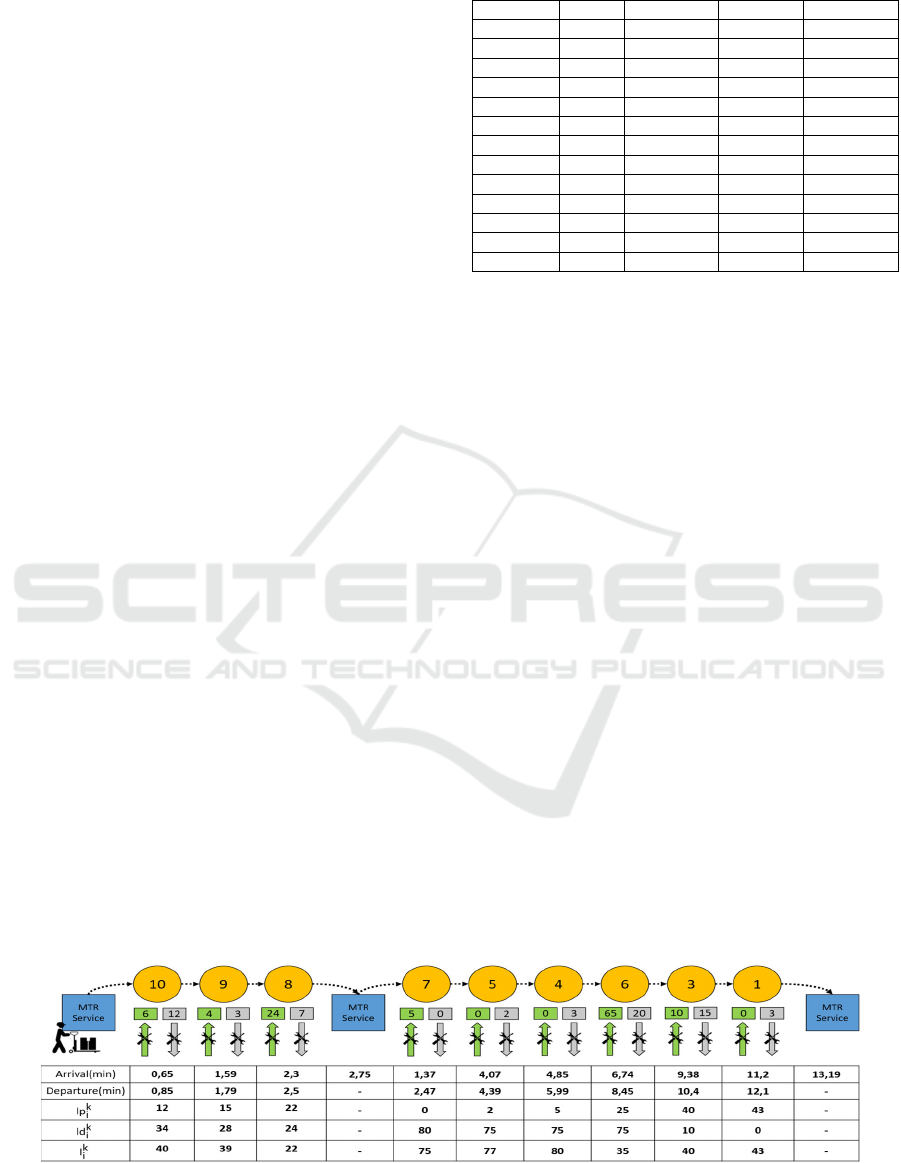
instance. Figure 3 presents a diagram with the 1
st
instance solution representation for the manual
vehicle. The yellow circles represent the customers,
and the blue square the depot. In green, we can see
the number of tools delivered to each customer and in
grey, the pickup quantities. Below the diagram, a
table with the following information is presented:
Vehicle’s arrival time at customer;
Vehicle’s departure time from customer;
Picked load after leaving the customer (𝑙𝑝
);
Load to be delivered to the customer and the
following customers (𝑙𝑑
);
Total load after the vehicle leaves the customer
( 𝑙
).
Figure 3: Solution of the 1
st
instance for the manual vehicle.
ICORES 2022 - 11th International Conference on Operations Research and Enterprise Systems
158
Table 5: MILP results for the automatic vehicle.
Instance Trips OF (min) CPU (s) GAP (%)
1 2 6.96 2.97 10.69
2 2 6.4 2.08 20.19
3 1 5.62 0.72 6.05
4 1 5.62 0.28 0
5 1 5.62 0.61 3.91
6 2 6.96 8.36 12.5
7 1 5.62 0.34 0
8 1 5.62 0.39 0
9 1 5.62 0.42 6.41
10 1 5.62 0.53 4
11 5 12.09 169.58 0.91
12 4 9.93 12.42 18.17
13 4 9.93 20.3 13.59
The total travel time, which includes the arcs
travel times, the service time and possible waiting
times, for this route is 13.19 minutes, and the MTR
worker needs to go 2 times to the depot, due to the
lack of vehicle’s capacity. With the current service
organisation, the workers need 26 minutes to do the
same service. This means that we reduced the time
consumed by 49%. It is important to note that, even
for the worst-case instances, the approach obtains a
smaller travel time than the company’s current one
for normal demand values. For the automatic vehicle,
we have in average a 14% reduction compared to the
current time for the same demand.
Vehicle-flow model efficiency test and time
windows sensitivity analysis. To test the model’s
efficiency in more challenging problem instances, the
adapted benchmarks from Li and Lim (2001) were
used. These problems’ objective is to minimise the
number of vehicles or routes. Due to the size of those
instances, only the first 20 customers of each instance
(IC2, IR2 and IRC2) were considered and adapted to
a VRPSDPTW. The results are presented in Table 6.
If the optimal solution is not reached within a pre-
defined time limit (10 minutes), the costs’ column
shows the best integer solution, and the CPU displays
a “-”. Like in the real problems (section 5.1), the
results in terms of solution GAP are not so good.
According to the problems’ characteristics, the CPU
time is relatively low. For the IRC problems, the
optimal solution was not achieved for the last 2
instances, within the time limit.
A time windows sensitivity analysis using the
automatic vehicle data was also performed. The tests
were made by reducing the time windows range. The
size of the time windows decreases from Case 1 to
Case 5. The results (Table 7) show that for tighter
time windows, the GAP becomes smaller. However,
this only happens until a certain point. This is,
because of the reduced time windows, one single
Table 6: Model results for the adapted benchmark problem
instances.
Instances
Vehicle-Flow Model
Costs CPU (sec) GAP (%)
IC201 252 0.01 0
IC202 202 1.69 11.88
IC203 194 8.69 2.36
IC204 186 4.01 0.96
IC205 251 0.75 1.40
IC206 230 1.64 3.28
IC207 218 1.89 1.87
IC208 205 3.74 3.78
IR202 399 46.84 0.87
IR203 354 91.19 0.71
IR204 289 42.68 0.81
IR205 350 1.86 1.19
IR206 318 11.4 2.83
IR207 318 61.82 0.69
IR208 260 2.53 1.08
IR209 312 3.87 2.26
IR210 353 79.06 0.69
IR211 293 253.83 0.46
IRC202 341 156.23 3.16
IRC203 309 - 20.95
IRC204 268 - 17.91
vehicle is no longer sufficient to make the route, not
because of capacity, but because the depot TW (Case
5). Also, when the TW are small (Case 4 and 5), the
OF values increase by 11% and 32%, respectively.
This can be related to the need to meet the TW, which
results in a visiting order that is not as efficient in
terms of travel distance.
Table 7: Time Windows Sensitivity analysis.
Case Trips OF (min) CPU (s) GAP (%)
Case 1 1 5.02 1.13 21.71
Case 2 1 5.02 1.22 18.63
Case 3 1 5.02 0.58 14.69
Case 4 1 5.62 1.42 10.50
Case 5 2 7.33 1.45 21.25
6 CONCLUSION AND FUTURE
WORK
A real-world problem of a Manufacturing Tool
Repair Support Service of an automotive company is
presented. One of the most time-consuming activities
performed by this service consists in the P&D of the
company’s manufacturing tools. Therefore, to
minimize this time and to increase service efficiency,
we modelled problem as a VRPSDPTW and solved
it. The stock levels in the production lines, together
with the number of repaired tools, are constantly
monitored and processed. Hence, when needed, the
MILP model generates routes with the sequence of
customers to visit and the related tools to P&D. Also,
Optimizing Route Planning for Minimising the Non-added-Value Tasks Times: A Simultaneous Pickup-and-Delivery Problem
159

compared to the current situation, the presented work
shows that, by using this approach, we can reduce up
to 49% the total travel time for one vehicle and 14%
for the other. Even in a worst-case scenario, the model
best results than the current ones for both vehicles. To
further improvements a 3-dimentional packing
problem integrated with the P&D problem is under
study.
REFERENCES
Gupta, A., Heng, C. K., Ong, Y. S., Tan, P. S., & Zhang, A.
N. (2017). A generic framework for multi-criteria
decision support in eco-friendly urban logistics systems.
Expert Systems with Applications, 71, 288–300.
Hof, J., & Schneider, M. (2019). An adaptive large
neighborhood search with path relinking for a class of
vehicle-routing problems with simultaneous pickup and
delivery. Networks, 74(3), 207–250.
Ji, Y. (2019). Optimal Scheduling in Home Health Care. In
ACM International Conference Proceeding Series (pp.
1–6).
Kumar, S. N., & Panneerselvam, R. (2012). A Survey on
the Vehicle Routing Problem and Its Variants,
2012(03), 66–74.
Lagos, C., Guerrero, G., Cabrera, E., Moltedo, A., Johnson,
F., & Paredes, F. (2018). An improved Particle Swarm
Optimization Algorithm for the VRP with
Simultaneous Pickup and Delivery and Time Windows,
16(6), 1732–1740.
Li, Haibing, & Lim, A. (2001). A metaheuristic for the
pickup and delivery problem with time windows.
Proceedings of the International Conference on Tools
with Artificial Intelligence, 160–167.
Li, Hongye, Wang, L., Hei, X., Li, W., & Jiang, Q. (2018).
A decomposition-based chemical reaction optimization
for multi-objective vehicle routing problem for
simultaneous delivery and pickup with time windows.
Memetic Computing, 10(1), 103–120.
Li, L., Li, T., Wang, K., Gao, S., Chen, Z., & Wang, L.
(2019). Heterogeneous fleet electric vehicle routing
optimization for logistic distribution with time windows
and simultaneous pick-up and delivery service. In 2019
16th International Conference on Service Systems and
Service Management, ICSSSM 2019. Institute of
Electrical and Electronics Engineers Inc.
Liu, S., Tang, K., & Yao, X. (2021). Memetic search for
vehicle routing with simultaneous pickup-delivery and
time windows. Swarm and Evolutionary Computation,
66(April), 100927.
Madankumar, S., & Rajendran, C. (2019). A mixed integer
linear programming model for the vehicle routing
problem with simultaneous delivery and pickup by
heterogeneous vehicles, and constrained by time
windows. Sadhana - Academy Proceedings in
Engineering Sciences, 44(2), 1–14.
Romeira, B., Cunha, F., & Moura, A. (2021). Development
and Application of an e-Kanban System in the
Automotive Industry. In IEOM Monterrey 2021
Conference. Monterrey.
Shahabi-Shahmiri, R., Asian, S., Tavakkoli-Moghaddam,
R., Mousavi, S. M., & Rajabzadeh, M. (2021). A
routing and scheduling problem for cross-docking
networks with perishable products, heterogeneous
vehicles and split delivery. Computers and Industrial
Engineering, 157(February), 107299.
Solomon, M. M. (1987). Algorithms for the Vehicle
Routing and Scheduling Problems with Time Window
Constraints.
Tang, K., Liu, S., Yang, P., & Yao, X. (2021). Few-Shots
Parallel Algorithm Portfolio Construction via Co-
Evolution. IEEE Transactions on Evolutionary
Computation, 25
(3), 595–607.
Wang, C., Mu, D., Zhao, F., & Sutherland, J. W. (2015). A
parallel simulated annealing method for the vehicle
routing problem with simultaneous pickup-delivery and
time windows. Computers and Industrial Engineering,
83, 111–122.
Wang, H. F., & Chen, Y. Y. (2012). A genetic algorithm for
the simultaneous delivery and pickup problems with
time window. Computers and Industrial Engineering,
62(1), 84–95.
Wang, J., Zhou, Y., Wang, Y., Zhang, J., Chen, C. L. P., &
Zheng, Z. (2016). Multiobjective Vehicle Routing
Problems with Simultaneous Delivery and Pickup and
Time Windows: Formulation, Instances, and
Algorithms. IEEE Transactions on Cybernetics, 46(3),
582–594.
Zhang, M., Pratap, S., Zhao, Z., Prajapati, D., & Huang, G.
Q. (2020). Forward and reverse logistics vehicle routing
problems with time horizons in B2C e-commerce
logistics. International Journal of Production
Research, 0(0), 1–20.
Zhou, Y., Kong, L., Cai, Y., Wu, Z., Liu, S., Hong, J., & Wu,
K. (2020). A Decomposition-Based Local Search for
Large-Scale Many-Objective Vehicle Routing Problems
with Simultaneous Delivery and Pickup and Time
Windows. IEEE Systems Journal, 14(4), 5253–5264.
ICORES 2022 - 11th International Conference on Operations Research and Enterprise Systems
160
