Efﬁcient Removal of Weak Associations in Consensus Clustering

N. C. Ruckiya Sinorina, Howard J. Hamilton

and Sandra Zilles

Department of Computer Science, University of Regina, 3737 Wascana Parkway, Regina, SK, Canada

Keywords:

Consensus Clustering, Association Matrix.

Abstract:

Consensus clustering methods measure the strength of an association between two data objects based on how

often the objects are grouped together by the base clusterings. However, incorporating weak associations in the

consensus process can have a negative effect on the quality of the aggregated clustering. This paper presents

an efﬁcient automatic approach for removing weak associations during the consensus process. We compare

our approach to a brute force method used in an existing consensus function, NegMM, which tends to be rather

inefﬁcient in terms of runtime. Our empirical analysis on multiple datasets shows that the proposed approach

produces consensus clusterings that are comparable in quality to the ones produced by the original NegMM

method, yet at a much lower computational cost.

1 INTRODUCTION

Consensus clustering refers to the process of generat-

ing an aggregation or ensemble of several individual

clusterings of a dataset, called base clusterings. Typ-

ically, in consensus clustering the ﬁnal clusters are

based on how frequently the data objects are grouped

together in the base clusterings (Strehl and Ghosh,

2003). Such techniques have been used in a broad

range of applications, including image processing,

network analysis, business process management, and

cloud computing (Wu et al., 2018). Other than cre-

ating robust and high-quality ﬁnal clusters, consensus

clustering supports distributed data mining, data pri-

vacy (Chalamalla, 2010), and knowledge re-usability.

To ﬁnd a common ground of agreement, some

consensus approaches analyze the association of data

objects to each other (Fred and Jain, 2005; Strehl and

Ghosh, 2003; Zhong et al., 2019). An association in-

dicates that a pair of data objects occur together in

a cluster, in some or all input base clusterings. Some

consensus functions examine each data object pair for

associations and form a pairwise association matrix

to generate the ﬁnal clusterings (Fred and Jain, 2005;

Strehl and Ghosh, 2003; Zhong et al., 2019). The val-

ues in an association matrix range from 0 to 1 based

on the frequency with which a data object pair is clus-

tered together in the base clusterings. An association

is weak if the frequency of a pair of data objects to oc-

https://orcid.org/0000-0003-1475-0980

https://orcid.org/0000-0001-7834-8574

cur in the same cluster is low, and the majority of base

clusterings keep the two objects in separate clusters.

Several consensus functions use association matrices

without distinguishing between strong and weak asso-

ciations; instead they treat each non-zero association

value as an association to take into account in cal-

culating a ﬁnal consensus clustering (Fred and Jain,

2005; Strehl and Ghosh, 2003).

Recently it was shown that removing weak asso-

ciations during consensus clustering can improve the

quality of the result (Baller et al., 2018; Zhong et al.,

2019). But how can one make a clear distinction

of weak and strong pairwise associations in the base

clusterings? In other words, which threshold value in

the interval from 0 to 1 should be the largest associ-

ation value below which the associations are consid-

ered weak? We call such value a weak association

threshold, and the problem of choosing it the thresh-

old selection problem. It is usually hard to answer

the above question in advance, and the best threshold

value will in general depend on the dataset and the

base clusterings (Baller et al., 2018).

To the best of our knowledge, the only existing

consensus method that attempts to solve the threshold

selection problem is NegMM (Zhong et al., 2019). It

is a brute force method that tests about 50 threshold

values and generates consensus candidates for all of

them. One of these consensus candidates is then cho-

sen as the ﬁnal output. Since NegMM searches for the

best weak association threshold among a large num-

ber of candidates, each time invoking the consensus

326

Sinorina, N., Hamilton, H. and Zilles, S.

Efﬁcient Removal of Weak Associations in Consensus Clustering.

DOI: 10.5220/0010820800003116

In Proceedings of the 14th International Conference on Agents and Artiﬁcial Intelligence (ICAART 2022) - Volume 3, pages 326-335

ISBN: 978-989-758-547-0; ISSN: 2184-433X

mechanism, it is computationally expensive.

In this paper, we address the question whether it

is possible to select a weak association threshold au-

tomatically based on the distribution of values in the

association matrix for a set of base clusterings con-

sidered for consensus, without exhaustively probing a

large number of thresholds. We propose an approach,

called the WAT (Weak Association Threshold) ap-

proach, to solve the threshold selection problem by

computing a threshold value based on the distribu-

tion of association values. In particular, our approach

is to apply a standard clustering algorithm (e.g., K-

Means (Aggarwal and Reddy, 2014) or Gaussian Mix-

ture Model clustering (Reynolds, 2015)) on the set of

association values, group the latter into two clusters,

and use the threshold value that separates these two

clusters as our weak association threshold.

In an empirical analysis on 16 datasets, we com-

pare the original NegMM method to two variants that

use our WAT approach in place of the brute force

threshold search. Our observations strongly suggest

that similar quality clusterings can be obtained with

much reduced computational cost when using the

WAT approach instead of generating numerous con-

sensus candidates in the original NegMM consensus

function.

2 RELATED WORK

Several procedures for aggregating clusterings for a

dataset have been proposed over the years. This pa-

per primarily focuses on consensus functions based

on pairwise associations. To combine the base clus-

terings and ﬁnd the aggregated result, such consensus

functions measure the similarity of two data points or

clusters in the base clusterings (Vega-Pons and Ruiz-

Shulcloper, 2011). To measure this similarity, these

methods consider the incidence of the pair grouped

in the same cluster by different clustering methods.

A convenient and effective representation of the pair-

wise data similarity measure is the association matrix

(Fred and Jain, 2005). With data points as rows and

columns, the values in this association matrix indi-

cate how many times a pair of objects are grouped in

the same cluster in the given base clusterings relative

to the total number of base clusterings considered for

consensus.

Fred and Jain proposed generating consensus re-

sults based on an association matrix using the Evi-

dence Accumulation method (EAC). It applies single-

linkage agglomerative clustering over an association

matrix of base clusterings to generate the consensus

(Fred and Jain, 2005).

Such an association matrix is a summary repre-

sentation of the participating base clusterings. As the

consensus function runs, evidence is accumulated in

the association matrix and the quality of the ﬁnal con-

sensus depends on the information in this representa-

tion. For example, the existence of many uncertain

data pairs in an association matrix can affect the ﬁ-

nal consensus. Uncertain data pairs are pairs that are

clustered together in about half of the base clusterings

and separated in the other half.

The problem of uncertain data pairs is addressed

in (Yi et al., 2012), by proposing the creation of a par-

tially observed association matrix, with reliable val-

ues only for the data pairs whose cluster memberships

are agreed upon by most of the clustering algorithms.

A matrix completion algorithm completes the matrix

and then applies spectral clustering to generate the ﬁ-

nal consensus. This approach deﬁnes a lower bound

of 0.2 and an upper bound of 0.8 for an association

value to be treated as uncertain. These thresholds may

not be ideal across all datasets and base clusterings.

Recently the NegMM consensus was proposed,

which removes weak associations from the associa-

tion matrix (Zhong et al., 2019). Evidence that occurs

in lower frequency in base clusterings is considered

as negative information, and treated as noise in the

association matrix. Including this negative evidence

between data objects is demonstrated to cause unde-

sirable effects in the consensus and degrade the con-

sensus performance (Zhong et al., 2019). Removing

weak associations means to decrease the frequency of

such undesired pairs in the association matrix. The

authors recommend removing small similarity values,

where the threshold for a weak association value lies

in the range from 0.01 to 0.5. NegMM consensus con-

siders all the values in this range, with an increment

of 0.01, as potential weak association thresholds. The

basic idea of NegMM consensus is to generate sev-

eral candidate consensus clusterings by removing the

weak associations using each possible threshold value

one at a time. The best clustering among the candi-

dates is then selected using a clustering internal va-

lidity measure. The details are discussed in Section 3.

The NegMM consensus function relies on a pre-

deﬁned set of thresholds to remove weak associations

during consensus. In our work, the main distinctive

feature is to deploy methods that can select a weak

association threshold without evaluating an extensive

set of candidates. We propose two ways of select-

ing weak association thresholds and explore which

method performs well under which conditions.

Efﬁcient Removal of Weak Associations in Consensus Clustering

327

Input : Base clusterings for dataset with n

objects, number of clusters K

Output: Final clustering C

∗

Generate an n ×n pairwise association matrix

of base clusterings, AM;

Initialize Candidates =

thresholds = {0,0.01,0.02,...,0.5};

for τ ∈thresholds do

∗

= AM;

if AM

∗

i j

≤ τ then

∗

i j

= 0;

end

= Ncut(AM

∗

,K);

Candidates = Candidates ∪C

;

end

Evaluate MM index for each

∈Candidates;

Return C

∗

= C

where C

∈Candidates

minimizes MM index;

Algorithm 1: Algorithm for NegMM consensus.

3 NegMM CONSENSUS

NegMM consensus is the “Negative Evidence Re-

moved Clustering Ensemble”, in which associations

of data pairs with low co-occurrence frequency in the

base clusterings are removed from the association ma-

trix (Zhong et al., 2019). Algorithm 1 displays the

method for NegMM consensus. It initially generates

a data-based association matrix using the input base

clusterings (line 1). For a dataset with n objects, using

z base clusterings P = {P

,..,P

}, an n×n data-based

association matrix AM is generated using

i j

= α(x

)/z (1)

where α(x

) is the number of times x

and x

oc-

cur together in the same cluster, across all base clus-

terings in P. NegMM considers all data pairs with

association values at most 0.5 as potentially weak as-

sociations. Weakly associated data points may appear

in two different clusters of the original base cluster-

ings, and such associations can be negative evidence

for consensus. However, as it is not easy to decide

which association evidence is negative information in

the matrix and ought to be removed, NegMM gradu-

ally removes association evidence within the range of

0 to 0.5, with an increase of 0.01 in each step. All as-

sociation values below the selected value in each step

are set as zeros to generate a modiﬁed association ma-

trix (lines 4 to 7). Then, normalized cut (Ncut) (Shi

and Malik, 2000) is applied over each of these mu-

tated association matrices, to generate candidate con-

sensus clusterings (line 8). Ncut is a graph partition-

ing algorithm – often applied for instance in image

segmentation – that uses a normalized cut criterion to

form the partitions, where the associations of edges

within the partitions of the graph are used for normal-

izing the cut. The reader is referred to (Shi and Malik,

2000) for more details on Ncut.

Among these candidate consensus clusterings, the

highest quality one is selected as the ﬁnal output clus-

tering, using a minimax similarity-based index (MM

index, lines 11 to 12). The MM index is an inter-

nal validity index to assess the quality of a clustering

(Zhong et al., 2019), that can be calculated without

accessing the original dataset. It deﬁnes a good clus-

tering as one in which the clusters have high stability

and low cohesion with other clusters. For a clustering

C = {C

,...,C

} with K clusters, the MM index is

deﬁned as follows.

MM =

∑

i=1

coh(C

,X \C

)/stb(C

) (2)

where coh(C

) is the cohesion between clusters C

and C

and stb(C

) is the stability of cluster C

in terms

of density-based connectivity (Zhong et al., 2019).

Cohesion and stability are given by

coh(C

,X \C

) = max

∈C

∈X\C

RS(x

,l)(3)

stb(C

) = min

∈C

RS(x

,l) (4)

where “\” denotes the set difference, and C

and C

are created by bi-partitioning C

, here using Ncut. For

an undirected graph G(X,E) over a data set X, with

similarity matrix S

, RS is the robust minimax sim-

ilarity value. This robust path-based minimax simi-

larity measure for x

and x

with l as the number of

nearest neighbours is deﬁned as

RS(x

,l) (5)

= max

p∈ρ

{ min

1≤h<|p|

sim(p[h], p[h + 1])w

h+1

} (6)

where ρ

is set of all paths between x

and x

, p[h] is

the h

vertex in path p, sim(x

) is the similarity of

and x

from S

, and w

is the weight for x

(Zhong

et al., 2019).

Increased stability indicates a high within-cluster

density and low cohesion indicates a low density-

based connectivity to other clusters. The MM index

favours clusterings that correspond to high-density re-

gions separated by low-density regions (Zhong et al.,

2019).

ICAART 2022 - 14th International Conference on Agents and Artiﬁcial Intelligence

328

Input : Base clusterings for dataset with n

objects

Output: n ×n pairwise association matrix

∗

without weak associations

Generate n ×n pairwise association matrix of

base clusterings, SM. Initialize i = 0, j = 0;

Let X be a sorted array of values in SM

greater than zero;

Generate two clusters in X using a clustering

algorithm;

select the maximum value in the left cluster

as τ;

while i < n and j < n do

if SM

i j

≤ τ then

∗

i j

= 0;

else

∗

i j

= SM

i j

;

end

Algorithm 2: Algorithm to remove weak associations.

4 APPROACH

Figure 1 gives an overview of the consensus process.

Our proposed WAT approach towards the threshold

selection problem is to apply a standard clustering al-

gorithm on the association values, thus cluster the as-

sociation values into two clusters, and use this two-

way clustering to derive a weak association threshold

τ. This paper tests the WAT approach with two clus-

tering techniques that are applied to the association

values, namely K-Means and Gaussian Mixture Mod-

els (GMM), to select the threshold τ automatically.

Algorithm 2 gives the general method. Initially,

one generates the pairwise association matrix of com-

ponent pairs in the base clusterings. With a dataset of

n objects, Algorithm 2 generates an n ×n data-based

association matrix SM (line 1). It then groups the as-

sociation values in the matrix into two clusters using

a basic clustering algorithm. These two clusters sep-

arate the larger association values in the matrix from

the smaller ones. The cluster that contains the mini-

mum association value that is greater than zero is re-

ferred to as the left cluster, and the cluster that con-

tains the maximum association value is referred to as

the right cluster. The highest value in the left cluster

is the cut-off value for the association value groups

and is the weak association threshold τ (line 4).

In our experiments, we tested two methods for

obtaining the required grouping of association values

into two clusters :

• K-Means with K = 2

• Gaussian Mixture Model Clustering using the EM

algorithm to model the set of association values as

a mixture of two Gaussians.

One sets all the values less than or equal to the

selected threshold to zero in the pairwise association

matrix (lines 5 to 10). The consensus is then gen-

erated using the new association matrix without the

weak associations. See Figure 2 for the K-Means

clusters and the Gaussians for the histogram of associ-

ation values for a synthetic dataset called Jain (Fr

anti

and Sieranoja, 2018).

The proposed way of removing the weak associa-

tions can be used with any consensus function that op-

erates on an association matrix, such as, for example

NegMM or CSPA (Strehl and Ghosh, 2003). This pa-

per analyzes the approach empirically in the context

of the NegMM consensus function. Instead of gen-

erating several consensus candidates, using the WAT

approach in the NegMM consensus function means to

ﬁrst calculate the threshold to remove weak associa-

tions and then to perform the consensus only with the

derived weak association threshold.

5 EMPIRICAL ANALYSIS

5.1 Experimental Datasets and

Implementation Details

The basic details of 16 datasets used in our exper-

iments, both real-world and synthetic, are given in

Table 1. The Blobs dataset with isotropic Gaussian

blobs for clustering analysis is generated using the

make blobs function with default parameters in Scikit

learn (Pedregosa et al., 2011). For evaluation pur-

poses, the datasets are all classiﬁcation datasets with

ground truth labels. The experiments are run on a

Windows OS computer with an Intel(R) Xeon(R) E3

processor, running at 3.70 GHz, and 8 GB of RAM.

All implementations are done in Python 3.7.

We experimented with four different sets of base

clusterings per dataset. In three of these four setups,

the mechanism for generating base clusterings is us-

ing multiple initializations of the K-Means clustering

algorithm. The experiments in this paper use the K-

Means implementation in Scikit-learn with parame-

ters n clusters, the number of clusters K set as de-

scribed below, max iter, the maximum number itera-

tions set to 4 instead of the default value of 300, and

n init, the number of restarts set to 1 instead of the de-

fault value of 10 (Pedregosa et al., 2011). Small val-

ues are used for max iter and the number of restarts to

increase the diversity of the clusterings produced by

Efﬁcient Removal of Weak Associations in Consensus Clustering

329

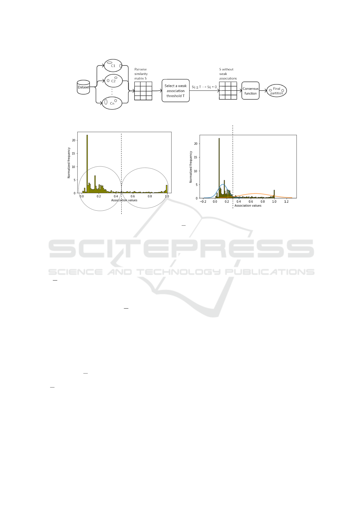
Figure 1: General overview of consensus clustering with removal of weak associations.

Figure 2: Histograms of data point association values obtained using 100 base clusterings on the Jain dataset. The base

clusterings were formed by K-Means clustering with K =

√

N and number of iterations set to 4. The dotted vertical line

separates the association values into two clusters, as determined by 2-Means (left) and GMM (right). The weak association

thresholds are 0.46 (left) and 0.33 (right).

the multiple initializations. All other parameters used

are defaults.

Setup 1: 1000 Base Clusterings, K-Means with K =

√

Nc. To create similar experimental settings as in

the original article on NegMM (Zhong et al., 2019),

a set of 1000 base clusterings is generated for each

dataset where K-Means is run 1000 times, with the

number of clusters K ﬁxed as b

√

Nc, for a dataset with

N instances.

Setup 2 (Resp. 3): 100 (Resp. 10) Base Clusterings,

K-Means with Random K. To investigate the effect

of using the proposed WAT approach over different

consensus sizes, this paper tests consensus functions

using 100 and 10 base clusterings separately, for all

datasets. Here, K-Means is run with random K rang-

ing from 2 to

√

N with the assumption that the appro-

priate number of clusters in a dataset will be at most

√

N (Bezdek and Pal, 1998).

Setup 4: 10 Diverse Base Clusterings. More di-

verse base clusterings are expected to be obtained by

using a variety of clustering algorithms to generate the

base clusterings. We generate 10 base clusterings for

each dataset by using 10 methods: (1) K-Means (Ag-

garwal and Reddy, 2014), (2) Mini Batch K-Means

(Sculley, 2010), (3) the density based clustering algo-

rithm DBSCAN (Aggarwal and Reddy, 2014), (4-6)

hierarchical agglomerative clustering (Aggarwal and

Reddy, 2014) with its three linkage variations Ward,

Complete, and Average (Pedregosa et al., 2011), (7)

Mean Shift (Comaniciu and Meer, 2002), (8) BIRCH

(Zhang et al., 1997), (9) Gaussian Mixture (Aggarwal

and Reddy, 2014), and (10) Bayesian Gaussian Mix-

ture (Roberts et al., 1998).

The evaluation measure used to compare the clus-

terings are Adjusted Rand Index (ARI) (Hubert and

Arabie, 1985) and Adjusted Mutual Index (AMI)

(Vinh et al., 2010). The purpose of the WAT approach

is to remove weak associations in a substantially more

efﬁcient way than NegMM does, without suffering a

substantial loss of quality in the resulting consensus

clusterings. Therefore, we also recorded runtimes.

Below we use NegMM-WAT(K) (NegMM-

WAT(GMM), resp.) to denote the version of NegMM

when replacing the brute force threshold search by

our WAT method using K-Means with K=2 (using

GMM with 2 Gaussians resp.)

ICAART 2022 - 14th International Conference on Agents and Artiﬁcial Intelligence

330

Table 1: Basic details of the datasets used in our analysis where attributes deﬁne the dimensionality of the dataset.

Dataset #Objects #Attributes #Classes Type

Flame (Fr

anti and Sieranoja, 2018) 240 2 2 Synthetic

Path Based (PB) (Fr

anti and Sieranoja, 2018) 300 2 3 Synthetic

Jain (Fr

anti and Sieranoja, 2018) 373 2 2 Synthetic

Compound (CM) (Fr

anti and Sieranoja, 2018) 399 2 6 Synthetic

R15 (Fr

anti and Sieranoja, 2018) 600 2 15 Synthetic

Blobs 650 2 4 Synthetic

AG (Fr

anti and Sieranoja, 2018) 788 2 7 Synthetic

Iris (Dua and Graff, 2017) 150 4 3 Real

Wine (Dua and Graff, 2017) 178 13 3 Real

Image Segmentation (IS) (Dua and Graff, 2017) 210 19 7 Real

Seeds (Dua and Graff, 2017) 210 7 3 Real

Glass (Dua and Graff, 2017) 214 9 6 Real

User Knowledge Model (UKM) (Dua and Graff, 2017) 258 5 4 Real

Ecoli (Dua and Graff, 2017) 336 8 8 Real

Libras Movement (LM) (Dua and Graff, 2017) 360 90 15 Real

Yeast (Dua and Graff, 2017) 1484 8 10 Real

5.2 Experimental Results

Tables 2–5 compare the consensus functions

NegMM, NegMM-WAT(K), and NegMM-

WAT(GMM) in terms of ARI (left) and AMI

(right). For the WAT methods, the percentage of

increase or decrease compared to NegMM is shown

in parentheses. Avg Base refers to the average ARI or

AMI of the base clusterings, with standard deviation

in parentheses.

With 1000 K-Means base clusterings, using the

same setup as in the literature, all three consensus

functions, NegMM, NegMM-WAT(K), and NegMM-

WAT(GMM), produced clusterings of similar quality

in most cases. The ﬁnal clustering performance is ei-

ther the same or slightly improved in terms of ARI

and AMI values for NegMM-WAT(K) method, ex-

cept for the AG and IS datasets. For the AG dataset,

in this case, the AMI results are identical too. Now,

considering the results for the NegMM-WAT(GMM),

again the performance is the same or slightly im-

proved compared to that of the original NegMM, for

all datasets other than AG, where WAT(GMM) causes

a very small loss in quality.

This raises the question of whether similar obser-

vations can be made for more diverse sets of base

clusterings than those that were tested in (Zhong et al.,

2019). Our additional experiments using 100 and 10

base clusterings adopt the same experimental setup

except for setting the number K of clusters for K-

Means base clusterings randomly between 2 and

√

Varying the number of clusters in base clusterings in-

creases the diversity of the base clusterings.

Consensus results of 100 base clusterings in

this case, using NegMM, NegMM-WAT(K), and

NegMM-WAT(GMM), are given in Table 3. For the

Jain, R15, Iris, Wine, and Glass datasets, the ARI and

AMI values for all three consensus functions are the

same. For the Flame, PB, and Blobs datasets, using

the WAT methods on top of NegM gave slightly im-

proved values, but the differences were minor.

For the Seeds dataset, NegMM with WAT(K) has

the same result as NegMM, but, using NegMM with

WAT(GMM) improves the clustering by 190% and

68% for ARI and AMI, respectively. This is be-

cause the threshold selected by WAT(GMM) is 0.05,

whereas NegMM and WAT(K) selected the thresholds

0.4 and 0.44, respectively (see Figure 3). Though

NegMM’s best candidate clustering with the small-

est MM index is for threshold 0.4, the ARI and AMI

evaluations suggest that this clustering is inferior to

the clustering for threshold 0.05, in this case.

For the IS and CM datasets, the original NegMM

method outperformed the WAT variants in terms of

ARI and AMI. Possibly the distribution of association

values relates better to a clustering into more than two

groups, rather than one with two groups (as assumed

by our WAT approach). For example, see the asso-

ciation values of the 100 base clusterings in the IS

dataset, given in Figure 3. For the AG dataset, while

using WAT(GMM) decreases the clustering perfor-

mance, NegMM and NegMM-WAT(K) produce con-

sensus clusterings of the same quality.

When generating 10 base clusterings using K-

Means with independently randomly chosen values

for K, the consensus functions NegMM and NegMM-

WAT(K) and NegMM-WAT(GMM) produced compa-

rable results for the datasets Flame, CM, Iris, Wine,

Ecoli, and Yeast. The clustering quality improved

by using WAT methods for the UKM dataset and

Efﬁcient Removal of Weak Associations in Consensus Clustering

331

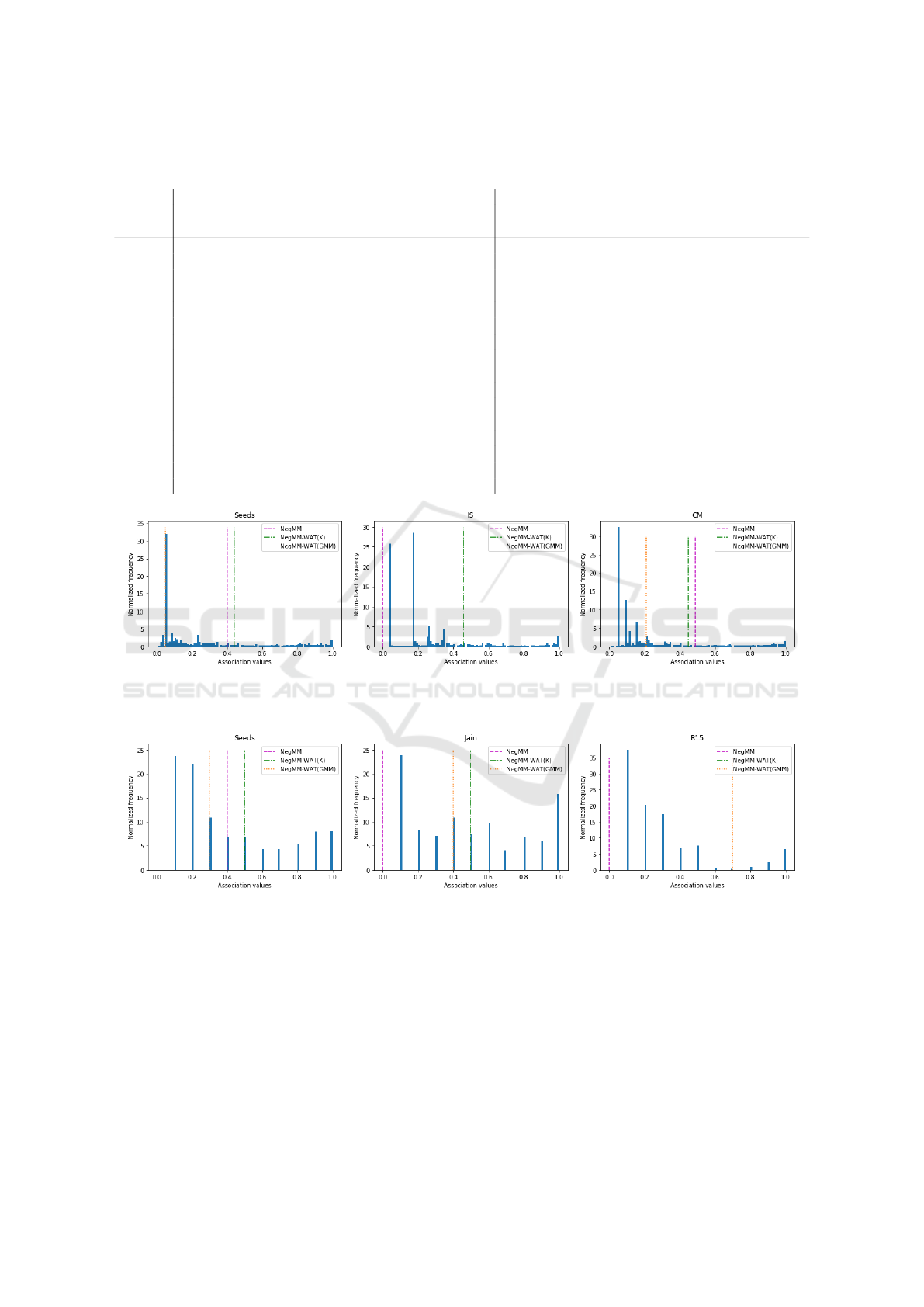
Table 2: Consensus results over 1000 base clusterings obtained from K-Means with ﬁxed K. The consensus functions

NegMM, NegMM-WAT(K), and NegMM-WAT(GMM) are compared in terms of ARI (left) and AMI (right).

ARI AMI

Dataset NegMM

NegMM

-WAT(K)

NegMM

-WAT(GMM)

Avg Base NegMM

NegMM

-WAT(K)

NegMM

-WAT(GMM)

Avg Base

Flame 0.45 0.45 (0%) 0.45 (0%) 0.45 (0.02) 0.4 0.4 (0%) 0.40 (0%) 0.40 (0.01)

PB 0.46 0.46 (0%) 0.46 (0%) 0.43 (0.05) 0.55 0.55 (0%) 0.55 (0%) 0.51 (0.05)

Jain 0.32 0.32 (0%) 0.32 (0%) 0.32 (0.01) 0.37 0.37 (0%) 0.37 (0%) 0.37 (0.01)

CM 0.54 0.54 (0%) 0.54 (0%) 0.54 (0.07) 0.72 0.72 (0%) 0.72 (0%) 0.71 (0.04)

R15 1 1.00 (0%) 1.00 (0%) 1.00 (0.00) 1 1.00 (0%) 1.00 (0%) 1.00 (0.00)

Blobs 0.82 0.82 (0%) 0.82 (0%) 0.82 (0.00) 0.84 0.84 (0%) 0.84 (0%) 0.84 (0.00)

AG 0.79 0.76 (-4%) 0.75 (-5%) 0.72 (0.04) 0.88 0.88 (0%) 0.87 (-1%) 0.84 (0.03)

Iris 0.72 0.73 (1%) 0.73 (1%) 0.73 (0.05) 0.74 0.76 (3%) 0.76 (3%) 0.75 (0.03)

Wine 0.37 0.37 (0%) 0.37 (0%) 0.36 (0.01) 0.43 0.43 (0%) 0.43 (0%) 0.43 (0.01)

IS 0.51 0.45 (-12%) 0.51 (0%) 0.40 (0.03) 0.66 0.65 (-2%) 0.66 (0%) 0.57 (0.03)

Seeds 0.72 0.72 (0%) 0.72 (0%) 0.71 (0.04) 0.69 0.69 (0%) 0.69 (0%) 0.70 (0.03)

Glass 0.54 0.55 (2%) 0.54 (0%) 0.49 (0.05) 0.74 0.74 (0%) 0.74 (0%) 0.70 (0.04)

UKM 0.17 0.17 (0%) 0.17 (0%) 0.19 (0.05) 0.26 0.27 (4%) 0.26 (0%) 0.26 (0.07)

Ecoli 0.42 0.42 (0%) 0.42 (0%) 0.43 (0.06) 0.62 0.62 (0%) 0.62 (0%) 0.60 (0.03)

LM 0.34 0.34 (0%) 0.34 (0%) 0.31 (0.02) 0.62 0.62 (0%) 0.62 (0%) 0.59 (0.01)

Yeast 0.13 0.13 (0%) 0.13 (0%) 0.13 (0.02) 0.26 0.25 (-4%) 0.26 (0%) 0.25 (0.02)

Figure 3: Plots for the distribution of NegMM-based association values for the Seeds, IS, and CM datasets with 100 base

clusterings. Different separators in the plot are where NegMM, NegMM-WAT(K), and NegMM-WAT(GMM), resp., put their

thresholds.

Figure 4: Distribution of NegMM-based association values of the Seeds, Jain, and R15 datasets with 10 K-Means base

clusterings. Different separators in the plot indicate where NegMM, NegMM-WAT(K), and NegMM-WAT(GMM) put their

thresholds, resp.

yielded slightly improved performance for the PB

and LM datasets, in terms of ARI and AMI values.

The WAT(K) method in this case for the Blobs and

Glass datasets also is comparable in performance to

NegMM. Using the NegMM-WAT(GMM) method,

for the dataset Seeds one obtains an improvement in

ARI by 21% and in AMI by 10%. The various thresh-

olds selected by the three consensus functions for the

Seeds dataset in this case, as shown in Figure 4, sug-

gests that WAT(GMM) selected the better threshold.

For both the Jain and the R15 dataset, from several

candidate clusterings, NegMM selected the clustering

with threshold 0 as its ﬁnal output and obtained per-

fect clusters (ARI and AMI are 1). That is, the con-

sensus of 10 random base clusterings for Jain and R15

identiﬁed the exact clusters in the datasets without re-

moving any associations. However, the WAT methods

selected thresholds near 0.5, as shown in Figure 4, for

ICAART 2022 - 14th International Conference on Agents and Artiﬁcial Intelligence

332

Table 3: Consensus results over 100 base clusterings obtained from K-Means with random K. The consensus functions

NegMM, NegMM-WAT(K), and NegMM-WAT(GMM) are compared in terms of ARI (left) and AMI (right).

ARI AMI

Dataset NegMM

NegMM

-WAT(K)

NegMM

-WAT(GMM)

Avg Base NegMM

NegMM

-WAT(K)

NegMM

-WAT(GMM)

Avg Base

Flame 0.93 0.95 (2%) 0.97 (4%) 0.23 (0.13) 0.88 0.90 (2%) 0.93 (6%) 0.49 (0.04)

PB 0.49 0.50 (2%) 0.50 (2%) 0.34 (0.09) 0.57 0.57 (0%) 0.57 (0%) 0.55 (0.04)

Jain 1 1.00 (0%) 1.00 (0%) 0.15 (0.07) 1 1.00 (0%) 1.00 (0%) 0.46 (0.04)

CM 0.64 0.48 (-25%) 0.54 (-16%) 0.40 (0.11) 0.8 0.70 (-13%) 0.72 (-10%) 0.70 (0.04)

R15 1 1.00 (0%) 1.00 (0%) 0.66 (0.27) 1 1.00 (0%) 1.00 (0%) 0.87 (0.12)

Blobs 0.8 0.82 (2%) 0.82 (2%) 0.37 (0.19) 0.83 0.84 (1%) 0.84 (1%) 0.65 (0.08)

AG 0.98 0.98 (0%) 0.78 (-20%) 0.43 (0.18) 0.98 0.98 (0%) 0.90 (-8%) 0.76 (0.07)

Iris 0.57 0.57 (0%) 0.57 (0%) 0.46 (0.13) 0.71 0.71 (0%) 0.71 (0%) 0.67 (0.04)

Wine 0.37 0.37 (0%) 0.37 (0%) 0.36 (0.01) 0.43 0.43 (0%) 0.43 (0%) 0.43 (0.01)

IS 0.46 0.40 (-13%) 0.40 (-13%) 0.32 (0.13) 0.59 0.58 (-2%) 0.58 (-2%) 0.52 (0.14)

Seeds 0.2 0.20 (0%) 0.58 (190%) 0.38 (0.13) 0.38 0.38 (0%) 0.64 (68%) 0.57 (0.04)

Glass 0.55 0.55 (0%) 0.55 (0%) 0.41 (0.14) 0.74 0.74 (0%) 0.74 (0%) 0.67 (0.08)

UKM 0.17 0.17 (0%) 0.17 (0%) 0.19 (0.06) 0.26 0.27 (4%) 0.26 (0%) 0.26 (0.07)

Ecoli 0.42 0.42 (0%) 0.4 (-5%) 0.42 (0.05) 0.62 0.62 (0%) 0.6 (-3%) 0.60 (0.02)

LM 0.32 0.32 (0%) 0.32 (0%) 0.23 (0.09) 0.6 0.60 (0%) 0.61 (2%) 0.48 (0.14)

Yeast 0.13 0.13 (0%) 0.13 (0%) 0.12 (0.02) 0.26 0.25 (-4%) 0.26 (0%) 0.25 (0.02)

Table 4: Consensus results over 10 base clusterings obtained from K-Means with random K. The consensus functions

NegMM, NegMM-WAT(K), and NegMM-WAT(GMM) are compared in terms of ARI (left) and AMI (right).

ARI AMI

Dataset NegMM

NegMM

-WAT(K)

NegMM

-WAT(GMM)

Avg Base NegMM

NegMM

-WAT(K)

NegMM

-WAT(GMM)

Avg Base

Flame 0.97 0.95 (-2%) 0.95 (-2%) 0.30 (0.14) 0.93 0.90 (-3%) 0.90 (-3%) 0.47 (0.06)

PB 0.44 0.47 (7%) 0.52 (18%) 0.37 (0.09) 0.53 0.52 (-2%) 0.59 (11%) 0.57 (0.04)

Jain 1 0.08 (-92%) 0.72 (-28%) 0.13 (0.05) 1 0.25 (-75%) 0.64 (-36%) 0.49 (0.04)

CM 0.54 0.54 (0%) 0.53 (-2%) 0.40 (0.08) 0.76 0.76 (0%) 0.76 (0%) 0.70 (0.03)

R15 1 0.79 (-21%) 0.83 (-17%) 0.63 (0.33) 1 0.93 (-7%) 0.90 (-10%) 0.84 (0.17)

Blobs 0.82 0.82 (0%) 0.64 (-22%) 0.43 (0.21) 0.84 0.84 (0%) 0.71 (-15%) 0.68 (0.09)

AG 0.99 0.92 (-7%) 0.72 (-27%) 0.38 (0.13) 0.99 0.93 (-6%) 0.87 (-12%) 0.77 (0.05)

Iris 0.57 0.57 (0%) 0.57 (0%) 0.50 (0.13) 0.71 0.71 (0%) 0.71 (0%) 0.68 (0.04)

Wine 0.37 0.37 (0%) 0.37 (0%) 0.37 (0.01) 0.43 0.43 (0%) 0.43 (0%) 0.43 (0.01)

IS 0.44 0.38 (-14%) 0.39 (-11%) 0.33 (0.13) 0.6 0.57 (-5%) 0.57 (-5%) 0.55 (0.08)

Seeds

0.48 0.43 (-10%) 0.58 (21%) 0.40 (0.16) 0.58 0.45 (-22%) 0.64 (10%) 0.58 (0.05)

Glass 0.53 0.54 (2%) 0.49 (-8%) 0.35 (0.1) 0.72 0.73 (1%) 0.69 (-4%) 0.66 (0.09)

UKM 0.18 0.26 (44%) 0.26 (44%) 0.23 (0.06) 0.26 0.32 (23%) 0.32 (23%) 0.30 (0.07)

Ecoli 0.42 0.43 (2%) 0.43 (2%) 0.44 (0.06) 0.6 0.6 (0%) 0.6 (0%) 0.59 (0.03)

LM 0.29 0.3.00 (3%) 0.31 (7%) 0.20 (0.11) 0.58 0.58 (0%) 0.59 (2%) 0.44 (0.17)

Yeast 0.14 0.13 (-7%) 0.14 (0%) 0.12 (0.03) 0.26 0.26 (0%) 0.26 (0%) 0.25 (0.03)

the same set of base clusterings, and the clustering

quality is not as good as that obtained by NegMM.

The last analysis uses 10 diverse base clusterings

obtained from multiple clustering algorithms. A con-

sensus over these base clusterings is again formed

using NegMM and NegMM-WAT(K). ARI and AMI

values of the ﬁnal clusterings are given in Table 5.

For most of the datasets, the NegMM-WAT(K)

consensus of these diverse 10 base clusterings gives

ﬁnal clusterings whose ARI and AMI values are com-

parable to those obtained by the original NegMM

method. For the Iris dataset, the AMI is unchanged,

but the ARI declines by 19%. Similarly, compar-

ing the WAT(GMM) results over those of the original

NegMM, for many datasets, the differences seemed

to be negligible. Interestingly, for the Glass dataset,

the clustering quality in terms of ARI improved by

37%, and for CM datasets by 9%. Also, the cluster-

ing quality of the Yeast data set improved using both

WAT methods in terms of ARI and AMI. In case of

Wine data set the threshold NegMM was able to pick

better threshold than WAT methods.

The runtime comparison of NegMM and its WAT

variants are shown in Figure 5. The NegMM consen-

sus involves a one-time generation of an association

matrix, multiple consensus steps to create candidate

clusterings, and selecting the best candidate as the ﬁ-

nal clustering. By contrast, the WAT approach run-

Efﬁcient Removal of Weak Associations in Consensus Clustering

333

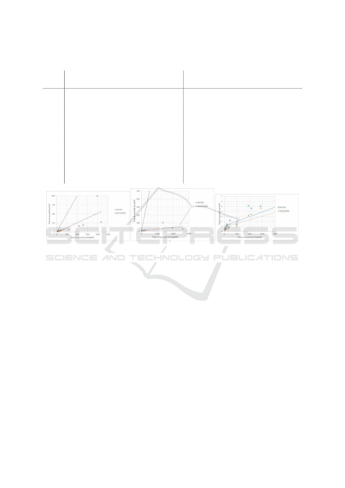
Table 5: Consensus results over 10 diverse base clusterings obtained from 10 clustering algorithms. The consensus functions

NegMM, NegMM-WAT(K), and NegMM-WAT(GMM) are compared in terms of ARI (left) and AMI (right).

ARI AMI

Dataset NegMM

NegMM

-WAT(K)

NegMM

-WAT(GMM)

Avg Base NegMM

NegMM

-WAT(K)

NegMM

-WAT(GMM)

Avg Base

Flame 0.45 0.45 (0%) 0.45 (0%) 0.27 (0.19) 0.46 0.46 (0%) 0.46 (0%) 0.32 (0.19)

PB 0.48 0.48 (0%) 0.48 (0%) 0.32 (0.22) 0.56 0.56 (0%) 0.56 (0%) 0.40 (0.23)

Jain 0.56 0.56 (0%) 0.56 (0%) 0.39 (0.36) 0.54 0.54 (0%) 0.54 (0%) 0.45 (0.27)

CM 0.57 0.57 (0%) 0.62 (9%) 0.63 (0.11) 0.71 0.71 (0%) 0.77 (8%) 0.74 (0.06)

R15 1 1.00 (0%) 1.00 (0%) 0.78 (0.27) 1 1.00 (0%) 1.00 (0%) 0.94 (0.08)

Blobs 0.81 0.81 (0%) 0.81 (0%) 0.75 (0.05) 0.83 0.83 (0%) 0.84 (1%) 0.85 (0.02)

AG 0.78 0.83 (6%) 0.80 (3%) 0.81 (0.07) 0.88 0.91 (3%) 0.88 (0%) 0.88 (0.04)

Iris 0.69 0.56 (-19%) 0.59 (-14%) 0.59 (0.20) 0.74 0.74 (0%) 0.62 (-16%) 0.69 (0.10)

Wine 0.91 0.55 (-40%) 0.55 (-40%) 0.55 (0.40) 0.89 0.68 (-24%) 0.68 (-24%) 0.62 (0.33)

IS 0.48 0.47 (-2%) 0.46 (-4%) 0.28 (0.20) 0.62 0.63 (2%) 0.61 (-2%) 0.50 (0.21)

Seeds 0.81 0.81 (0%) 0.81 (0%) 0.54 (0.35) 0.76 0.76 (0%) 0.76 (0%) 0.58 (0.27)

Glass 0.19 0.19 (0%) 0.26 (37%) 0.17 (0.14) 0.38 0.35 (-8%) 0.35 (-8%) 0.36 (0.14)

UKM 0.27 0.27 (0%) 0.27 (0%) 0.14 (0.13) 0.34 0.33 (-3%) 0.33 (-3%) 0.25 (0.15)

Ecoli 0.48 0.49 (2%) 0.47 (-2%) 0.38 (0.26) 0.61 0.63 (3%) 0.6 (-2%) 0.51 (0.16)

LM 0.31 0.31 (0%) 0.31 (0%) 0.19 (0.14) 0.6 0.59 (-2%) 0.59 (-2%) 0.48 (0.21)

Yeast 0.16 0.17 (6%) 0.17 (6%) 0.06 (0.07) 0.26 0.29 (12%) 0.28 (8%) 0.22 (0.12)

Figure 5: Runtime comparison of NegMM to NegMM-WAT(K), and NegMM to NegMM-WAT(GMM), using 1000, 100, and

10 base clusterings for datasets. Each point refers to one dataset. The dotted lines give the best ﬁts for the recorded data. The

solid line is the graph of y = x. In the rightmost graph the line for y = x is not shown, since with the chosen scales it would be

nearly identical to the y-axis, indicating a substantial runtime advantage of WAT over NegMM.

time involves creating the association matrix, select-

ing the threshold from the distribution, and the gener-

ation of a single consensus clustering. The trend line

in the scatter plot is the best ﬁt for the run-time data,

and it generalizes the observations.

The slope of the trend line for 1000 base cluster-

ings is 0.129, which means that NegMM consensus

takes about 7.7 times as much time as its WAT vari-

ants using 1000 base clusterings. Generally, the time

to create an association matrix is quadratic in the size

of the dataset and linear in the number of base clus-

terings used. With 1000 base clusterings, a consid-

erable portion of runtime for both the NegMM and

WAT variants is utilized for generating the matrix it-

self. Despite this, the rate of runtime difference is

noticeable.

The runtime plot for 100 base clusterings has trend

lines of even smaller slopes (around 0.012) compared

to that for 1000 base clusterings. The average ratio

indicates that NegMM takes about 51.4 times as much

time as its WAT variants using 100 base clusterings.

Using 10 base clusterings, on average NegMM takes

233 times as much time as its WAT variants.

Based on these results, we conclude that our WAT

approach yields noticeable runtime savings without

substantially reducing the clustering quality when

compared to NegMM in the experimental setting that

was originally tested in (Zhong et al., 2019). The run-

time savings increase with smaller consensus sizes,

while the clustering quality stays comparable to that

of NegMM, with a tendency to higher losses for

smaller consensus sizes.

6 CONCLUSION

The NegMM consensus function relies on removing

weak associations from the association matrix to im-

prove the ﬁnal clustering. This consensus function

is effective and outperforms other consensus function

to create high quality clusterings for many datasets

(Zhong et al., 2019). However, to select the best clus-

tering, NegMM generates several candidate cluster-

ICAART 2022 - 14th International Conference on Agents and Artiﬁcial Intelligence

334

ings, partially removing associations each time us-

ing a range of threshold values. The WAT approach

in combination with NegMM instead determines one

threshold, and generates the ﬁnal consensus directly.

Our empirical results for the majority of datasets over

different generation mechanisms and varied consen-

sus sizes suggest that the WAT approach is success-

ful in removing the weak associations to attain simi-

lar quality clusterings in much-reduced runtime com-

pared to the original NegMM method. This was evi-

dent in particular in our experiments with 1000 and

with 100 base clusterings. Further studies will be

needed to determine why the WAT approach hurt

the clustering performance of NegMM more in the

case of 10 less diverse base clusterings. Moreover,

the WAT approach surprisingly improved the qual-

ity of some NegMM clusterings, for example, apply-

ing WAT(GMM) for the consensus of 100 and 10 K-

Means base clusterings for the Seeds dataset.

ACKNOWLEDGEMENTS

Funding for this research was provided by ISM

Canada and the Natural Sciences and Engineering Re-

search Council of Canada.

REFERENCES

Aggarwal, C. C. and Reddy, C. K. (2014). Data Cluster-

ing: Algorithms and Applications. CRC Press, Boca

Raton, Florida, USA.

Baller, T., Hamilton, H., and Zilles, S. (2018). A meta ap-

proach to removing weak links during consensus clus-

tering. Unpublished manuscript.

Bezdek, J. C. and Pal, N. R. (1998). Some new indexes of

cluster validity. IEEE Transactions on Systems, Man

& Cybernetics. Part B (Cybernetics), 28(3):301–315.

Chalamalla, A. K. (2010). A survey on consensus cluster-

ing techniques. Technical report, Department of Com-

puter Science, University of Waterloo.

Comaniciu, D. and Meer, P. (2002). Mean shift: A robust

approach toward feature space analysis. IEEE Trans-

actions on Pattern Analysis and Machine Intelligence,

24(5):603–619.

Dua, D. and Graff, C. (2017). UCI machine learning repos-

itory. University of California, Irvine, School of Infor-

mation and Computer Sciences.

anti, P. and Sieranoja, S. (2018). K-means properties

on six clustering benchmark datasets. Applied Intel-

ligence, 48(12):4743–4759.

Fred, A. L. and Jain, A. K. (2005). Combining multiple

clusterings using evidence accumulation. IEEE Trans-

actions on Pattern Analysis and Machine Intelligence,

27(6):835–850.

Hubert, L. and Arabie, P. (1985). Comparing partitions.

Journal of Classiﬁcation, 2(1):193–218.

Pedregosa, F., Varoquaux, G., Gramfort, A., Michel, V.,

Thirion, B., Grisel, O., Blondel, M., Prettenhofer,

P., Weiss, R., Dubourg, V., Vanderplas, J., Passos,

A., Cournapeau, D., Brucher, M., Perrot, M., and

Duchesnay, E. (2011). Scikit-learn: Machine learning

in Python. Journal of Machine Learning Research,

12(85):2825–2830.

Reynolds, D. A. (2015). Gaussian mixture models. In Li,

S. Z. and Jain, A. K., editors, Encyclopedia of Biomet-

rics, pages 827–832. Springer, Boston, MA, USA.

Roberts, S. J., Husmeier, D., Rezek, I., and Penny, W.

(1998). Bayesian approaches to Gaussian mixture

modeling. IEEE Transactions on Pattern Analysis and

Machine Intelligence, 20(11):1133–1142.

Sculley, D. (2010). Web-scale K-means clustering. In

Proceedings of the 19th International Conference on

World Wide Web (WWW 2010), pages 1177–1178.

Shi, J. and Malik, J. (2000). Normalized cuts and image

segmentation. IEEE Transactions on Pattern Analysis

and Machine Intelligence, 22(8):888–905.

Strehl, A. and Ghosh, J. (2003). Cluster ensembles: A

knowledge reuse framework for combining multiple

partitions. Journal of Machine Learning Research,

3:583–617.

Vega-Pons, S. and Ruiz-Shulcloper, J. (2011). A sur-

vey of clustering ensemble algorithms. Intl. Jour-

nal of Pattern Recognition and Artiﬁcial Intelligence,

25(3):337–372.

Vinh, N., Epps, J., and Bailey, J. (2010). Informa-

tion theoretic measures for clusterings comparison:

Variants, properties, normalization and correction for

chance. Journal of Machine Learning Research,

11(2010):2837–2854.

Wu, X., Ma, T., Cao, J., Tian, Y., and Alabdulkarim, A.

(2018). A comparative study of clustering ensem-

ble algorithms. Computers & Electrical Engineering,

68:603–615.

Yi, J., Yang, T., Jin, R., Jain, A. K., and Mahdavi, M.

(2012). Robust ensemble clustering by matrix com-

pletion. In Proceedings of the 12th IEEE International

Conference on Data Mining, (ICDM 2012), pages

1176–1181.

Zhang, T., Ramakrishnan, R., and Livny, M. (1997).

BIRCH: A new data clustering algorithm and its ap-

plications. Data Min. Knowl. Discov., 1(2):141–182.

Zhong, C., Hu, L., Yue, X., Luo, T., Qiang, F., and Haiyong,

X. (2019). Ensemble clustering based on evidence ex-

tracted from the co-association matrix. Pattern Recog-

nition, 92:93–106.

Efﬁcient Removal of Weak Associations in Consensus Clustering

335