Error Evaluation of Semantic VSLAM Algorithms for Smart Farming

Adam Kalisz

1 a

, Mingjun Sun

1 b

, Jonas Gedschold

2 c

, Tim Erich Wegner

2 d

and Giovanni del Galdo

2,3 e

and J

orn Thielecke

1 f

Department of Electrical, Electronic and Communication Engineering, Information Technology (LIKE),

Friedrich-Alexander-Universit

at Erlangen-N

urnberg, Am Wolfsmantel 33, Erlangen, Germany

Institute for Information Technology, TU Ilmenau, Ehrenbergstraße 29, Ilmenau, Germany

Fraunhofer Institute for Integrated Circuits (IIS), Am Vogelherd 90, Ilmenau, Germany

Keywords:

Smart Farming, Semantic Segmentation, Visual, Localization, SLAM.

Abstract:

In recent years, crop monitoring and plant phenotyping are becoming increasingly important tools to improve

farming efﬁciency and crop quality. In the ﬁeld of smart farming, the combination of high-precision cameras

and Visual Simultaneous Localization And Mapping (SLAM) algorithms can automate the entire process from

planting to picking. In this work, we systematically analyze errors on trajectory accuracy of a watermelon ﬁeld

created in a virtual environment for the application of smart farming, and discuss the quality of the 3D mapping

effects from an optical point of view. By using an ad-hoc synthetic data set we discuss and compare the

inﬂuencing factors with respect to performance and drawbacks of current state-of-the-art system architectures.

We summarize the contributions of our work as follows: (1) We extend ORB-SLAM2 with Semantic Input

which we name SI-VSLAM in the following. (2) We evaluate the proposed system using real and synthetic

data sets with modelled sensor non-idealities. (3) We provide an extensive analysis of the error behaviours

on a virtual watermelon ﬁeld which can be both static and dynamic as an example for a real use case of the

system.

1 INTRODUCTION

In recent years, with the rapid development of indus-

trial automation and breakthroughs in Visual SLAM

technology, robots have been widely adopted in in-

dustrial production. Using agricultural robots com-

bined with technologies such as semantic segmenta-

tion, people can monitor the type and growth of crops

in real time (Ganchenko and Doudkin, 2019).

Our work is focused around developing a mobile,

multi-sensor crop monitoring system within a coop-

erative project between Technische Universit

at Ilme-

nau and Friedrich-Alexander-University of Erlangen-

Nuremberg. The aim of the project

is to build a

https://orcid.org/0000-0001-5428-5433

https://orcid.org/0000-0001-8943-817X

https://orcid.org/0000-0002-0251-887X

https://orcid.org/0000-0001-9484-7998

https://orcid.org/0000-0002-7195-4253

https://orcid.org/0000-0001-6671-6341

This contribution is partly funded by DFG project

420546347

universal system that can identify, map and monitor

any plant. This is also the motivation for creating

a virtual environment in which the speciﬁc charac-

teristics of different plant species can be tested and

evaluated. We have decided to use watermelons as a

ﬁrst example in our work as they exhibit easily recog-

nizable characteristics, such as changing colors, sizes

and textures during their growth process. One of the

main sensors used on our platform is a stereo (RGB-

D) camera. In order to provide farmers with a ro-

bust way to efﬁciently monitor their land, and thus

reduce waste and improve productivity, we need to

be aware of how erroneous measurements may im-

pact the quality of the mapping process. Inspired by

ORB-SLAM2 (Mur-Artal and Tard

os, 2017) and DS-

SLAM (Yu et al., 2018), this work proposes and sys-

tematically evaluates a Visual SLAM system which

utilizes semantic segmentation as its input. This sys-

tem is named Visual SLAM with Semantic Input (SI-

VSLAM) in the following.

In our research, we found that most of the seman-

tic SLAM projects are build on neural networks and

Kalisz, A., Sun, M., Gedschold, J., Wegner, T., Galdo, G. and Thielecke, J.

Error Evaluation of Semantic VSLAM Algorithms for Smart Farming.

DOI: 10.5220/0010820500003124

In Proceedings of the 17th International Joint Conference on Computer Vision, Imaging and Computer Graphics Theory and Applications (VISIGRAPP 2022) - Volume 5: VISAPP, pages

801-810

ISBN: 978-989-758-555-5; ISSN: 2184-4321

801

real data, such as DS-SLAM based on Caffe-SegNet

and semantic slam (Xuan and David, 2018) based on

PSPNet. However, they only analyzed the accuracy

of the trajectories through the TUM data set, and paid

little attention to the effects of the generated semantic

maps. Usually, the construction of a neural network

needs to collect a large number of pictures, which will

greatly increase the time cost. The neural network

itself may still output incorrect predictions due to a

representation bias (Li and Vasconcelos, 2019). Real

data sets also have some inconveniences. Most of the

existing public data sets, such as TUM and EuRoC, do

not provide semantic image sequences, and they can-

not be applied to smart farming. More importantly,

due to the randomness of environmental factors, it is

impractical to use real data sets to further analyze in-

dividual inﬂuencing factors in the environment. Con-

sidering the limitations of neural networks and real

data sets, we use the 3D scene simulation software

Blender

in order to create a custom synthetic agri-

cultural environment, namely a watermelon ﬁeld, and

use related plug-ins to generate perfect RGB, depth

and semantic image sequences. Then, by systemati-

cally deteriorating these image sequences using error

models from the literature, we investigate how each

error impacts both localization and mapping accu-

racy as it would in a real measurement. Additionally,

we test our system on slightly different environments,

both static and dynamic (e.g. moving objects), in or-

der to determine how plant growth / distribution may

inﬂuence the robustness of the system. Compared

with real data sets, synthetic scenes allow us to inde-

pendently control environmental variables in order to

discuss their effects on a speciﬁc SLAM system. This

contribution proposes methods for systematic analy-

sis of semantic SLAM systems using synthetic data

sets and thus beneﬁt the research community.

In the next section, we will brieﬂy describe the

design of the entire system and its individual compo-

nents. In the third section, we will introduce the setup

for a systematic evaluation, including the creation of

synthetic data sets and a series of experiments based

on these data sets. Finally, the whole work will be

summarized in the last section.

2 SYSTEM OVERVIEW

In this section, the framework of the system will be

introduced in detail. Figure 1 shows the ﬂow chart of

the system.

SI-VSLAM is a system based on ORB-SLAM2

https://www.blender.org/

RGB

Depth

Semantic

Remove dynamic

objects

RGB point cloud

Semantic point

cloud

Track

Visual

Odometry

RGB

Octomap

Semantic

Octomap

Figure 1: Flow chart of SI-VSLAM. We propose to extend

ORB-SLAM2 by an additional semantic input and to use

it in order to remove dynamic objects before tracking the

camera motion. Furthermore, we added three-dimensional

occupancy grid maps (octomaps) to the ﬁnal system (green

blocks).

(Mur-Artal and Tard

os, 2017). This work adds an

additional interface for the input of semantic images

to ORB-SLAM2, and adds the function of generating

dense point clouds. For subsequent visual compar-

ison, the generated semantic and RGB point clouds

will be saved to disk in order to be inspected sepa-

rately. The most commonly used map in robot nav-

igation and positioning is a 3D occupancy grid map,

and the octree map is one of the occupancy grid maps

based on the octree algorithm. If the Robot Operating

System (ROS) is used, this SLAM system can also

dynamically update the octree map in real time.

The authors of DS-SLAM proposed the idea of us-

ing optical ﬂow to detect dynamic objects and seman-

tic segmentation to eliminate unstable feature points.

By ﬁltering out unstable feature points, the robustness

and accuracy of the system can be signiﬁcantly im-

proved. However, this method of ﬁrst extracting fea-

ture points and then removing unstable points is risky.

When there are many dynamic objects in the scene,

this method may result in too few feature points left,

which is hardly conducive to the feature matching.

Differently from DS-SLAM, in SI-VSLAM the fea-

ture point extraction is performed after the dynamic

object is masked out in the image, so as to ensure that

there are enough feature points during feature match-

ing. Taking into account the impact of animals walk-

ing across the agricultural environment, we analyze

their inﬂuence on our system.

In 2020, ORB-SLAM3 (Campos et al., 2021) was

released, which added a ﬁsheye camera model to

the prior version. Furthermore, ORB-SLAM3 was

improved in the relocalization part, such as using

Multiple-Maps (ORBSLAM-Atlas), to recover when

the tracking is lost. Finally, ORB-SLAM3 also added

the ability of fusing Inertial Measurement Unit (IMU)

data. The reason why the latest version of ORB-

SLAM3 was not used in our work is that we are more

familiar with ORB-SLAM2 and do not necessarily re-

quire the new features for our experiments.

VISAPP 2022 - 17th International Conference on Computer Vision Theory and Applications

802

3 EVALUATION

The performance of a SLAM system can be analyzed

from multiple perspectives, such as time / space com-

plexity, power consumption and accuracy. Due to our

current plan to create and analyze the semantic maps

ofﬂine, after the system has been carried across the

ﬁeld by the farmer, we do not require fast or energy

efﬁcient processing at the moment. Therefore, we fo-

cus on the accuracy of the proposed system in this pa-

per. In this section, we will speciﬁcally introduce how

to use the synthetic data set to systematically evaluate

the SLAM system.

3.1 General Evaluation Metrics

The commonly used method is to use the absolute tra-

jectory error (ATE) or the relative pose error (RPE) to

evaluate the accuracy of the estimated camera trajec-

tory. ATE and RPE were deﬁned in the TUM data

set benchmark for the ﬁrst time and are widely used

(Sturm et al., 2012). After the initialization phase, a

global coordinate system is created on the basis of the

ﬁrst keyframe, the pose P

of the i-th frame is cal-

culated by Iterative Closest Point (ICP) and Bundle

Adjustment (BA) and this will be repeated until the

last camera frame n, such that the estimated poses are

, ..., P

∈ SE(3). The reference pose of the camera

is represented by Q

, which can be read directly from

the ground truth, Q

, ..., Q

∈ SE(3). A time interval

between two camera frames is represented by ∆. It is

assumed that the timestamp of the estimated poses is

aligned with the timestamp of the real poses and their

total number of frames is the same.

3.1.1 Relative Pose Error (RPE)

RPE mainly describes the accuracy of the pose differ-

ence between two frames with a ﬁxed time difference

∆ (compared to the real pose difference) (Prokhorov

et al., 2019). RPE of the i-th frame can be expressed

:= (Q

−1

i+∆

)

−1

i+∆

). (1)

The root mean square error (RMSE)

RMSE(E

1:n

, ∆) :=

∑

i=1

ktrans(E

, (2)

can be used to calculate the RPE of the entire system,

by using m = n −∆ individual RPEs. Note that Equa-

tion 2 only considers the translational components of

each RPE trans(E

). The rotation component gener-

ally does not need to be calculated, because the rota-

tional error increases the translational errors as well

when the camera is moved (Zhang and Scaramuzza,

2018).

3.1.2 Absolute Trajectory Error (ATE)

While the RPE allows to evaluate the drift per frame,

the ATE helps to evaluate the global consistency of

the estimated trajectory. The ATE compares the ab-

solute distances between the estimated pose and the

reference pose. It can very intuitively reﬂect the accu-

racy of the algorithm. The estimated pose and ground

truth in most cases are not in the same coordinate sys-

tem. Therefore, an approximation rigid-body trans-

formation S ∈ SE(3) can be calculated using least

squares methods prior to ATE calculations. The ATE

of the i-th frame can be represented by

:= Q

−1

. (3)

Similarly, the ATE of the entire system can also be

expressed as RMSE

RMSE(F

1:n

) :=

∑

i=1

ktrans(F

. (4)

In this work, ATE is used as the evaluation met-

ric of trajectory accuracy. Compared with RPE, ATE

is less computationally intensive and more sensitive.

In order to account for any randomness in the estima-

tions (for example caused by RANdom SAmple Con-

sensus, RANSAC, within ORB-SLAM2), all the cal-

culation results regarding trajectory accuracy in the

following are the average of 10 runs on the same in-

put.

3.2 Demonstration of Practicability and

Feasibility using the TUM Data Set

Before the speciﬁc analysis of the inﬂuencing factors,

real data sets must ﬁrst be used in order to check the

feasibility and practicability of the algorithm.

The TUM RGB-D benchmark is a popular data

set for RGB-D cameras and contains numerous im-

age sequences, each of which provides RGB images,

depth images and ground truth. In the experiment,

we selected three data sets, namely freiburg1 room

(F1), freiburg2 desk (F2) und freiburg3 walking xyz

(F3). Compared with the camera in F2, the camera in

F1 moves faster and has a wider range of movement.

With F3, the inﬂuence of dynamic objects on the sys-

tem can be discussed. Since there is no semantic pic-

ture sequence in the TUM dataset, dynamic objects

cannot be ﬁltered out. The accuracy of the algorithms

when running different image sequences is shown in

Figure 2.

Error Evaluation of Semantic VSLAM Algorithms for Smart Farming

803

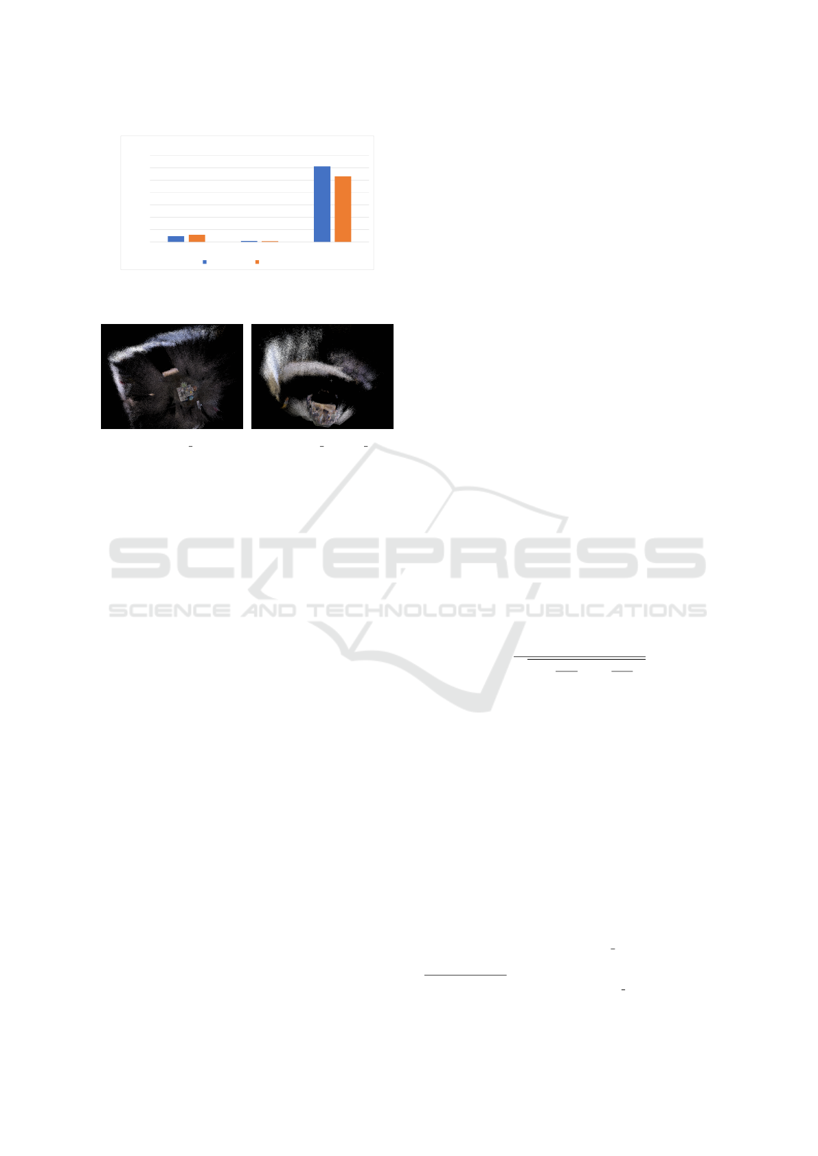
0.0476

0.0095

0.6104

0.0595

0.0077

0.5311

freiburg1_room freiburg2_desk freiburg3_walking_xyz

0.1

0.2

0.3

0.4

0.5

0.6

0.7

ATE (m)

Comparison on TUM Benchmark

ORB-SLAM2 SI-VSLAM

Figure 2: ATE of ORB-SLAM2 and SI-VSLAM when run-

ning on different picture sequences.

(a) freiburg2 desk. (b) freiburg3 walking xyz.

Figure 3: TUM RGB-D benchmark point clouds.

From Figure 2 it can be seen that ORB-SLAM and

SI-VSLAM have a high accuracy in a relatively static

environment, especially when the range of motion of

the camera is small and the speed of motion is slow. If

there are dynamic objects in the system and the area

of the dynamic objects is large, the accuracy of the

two systems will be severely affected.

The point clouds of F2 and F3 generated by SI-

VSLAM are shown in Figure 3a and 3b.

The update of the point cloud is a constant addi-

tion process. The point cloud of unstable objects and

the point cloud generated due to an incorrect pose

estimate remain in the map, making the map difﬁ-

cult to interpret. It can be seen from both ﬁgures

that the depth noise increases as the depth value in-

creases. This conclusion was proven by experiments

in the work Noise Modeling and Uncertainty Prop-

agation for Time of Flight (ToF) Sensors (Belhedi

et al., 2012).

3.3 Creation of Synthetic Data Sets

During this research, we found that most of the se-

mantic SLAM projects focus on the training of se-

mantic models and analyze the accuracy of object

recognition, but there is not much analysis of Visual

SLAM. One reason why this is difﬁcult, is that in a

real setting it is not trivial to independently control

the variables of the environment and thus evaluate

how neural network predictions are composed in de-

tail. Moreover, the SLAM part of the research is often

focused on trajectory analysis, and not enough atten-

tion is paid to the mapping. However, a SLAM system

is often affected by many factors, such as noise, light

intensity, and incorrect semantic segmentation, which

may threaten the robustness of the system. In order

to have a more systematic research on semantic map-

ping, we use Blender to build a synthetic agricultural

scene, and all simulation models are built according

to the existing literature.

3.3.1 Add-on: Vision-Blender

Vision-Blender

(Cartucho et al., 2020) is a synthetic

data set generator based on Blender 2.82. Vision-

Blender was specially developed for robotic surgery.

It can be used to create practical data sets for veriﬁ-

cation of computer vision algorithms, greatly reduc-

ing the cost required to prepare the data set. Vision-

Blender can extract the intrinsic parameters of the

camera, the pose of objects, calculate depth values

and provide the masks for the semantic segmentation.

Blender provides two rendering engines, Eevee

and Cycles. The semantic segmentation can only

be generated when the Cycles engine is used. Cy-

cles in Blender 2.82 uses path tracing for rendering.

The measurement model of the depth value is similar

to the model of the ToF sensor in RGB-D cameras,

which uses the end-to-end delay to measure distances

(Heckenkamp, 2008), therefore it uses the distance

along the line of sight (z

The distance model usually used in SLAM is the

vertical distance to the image plane (z), the depth

value must be corrected by a projection operation

z =

1 + (

−u

)

+ (

−v

)

, (5)

where f

, f

, c

are the intrinsic parameters of the

camera, u and v are the coordinates of the pixel in the

image. However, we found that the latest Blender (at

the time of this writing, version 2.93) has been im-

proved, and one no longer needs to modify the depth

value. Vision-blender can generate a large synthetic

data set where the artist can quickly specify the se-

mantic labels of objects in the scene. Consequently,

it has great potential to be applied in our experiments

where the robustness and mapping quality needs to be

thoroughly assessed.

3.3.2 Overview of the Synthetic Data Set

The experiments in this paper were conducted using

a custom data set with a length of 610 frames. The

basic data set is named 16plants static, which con-

tains 13 ripe watermelons, 10 unripe watermelons and

https://github.com/Cartucho/vision blender

VISAPP 2022 - 17th International Conference on Computer Vision Theory and Applications

804

16 plants. In the experiments, the RGB-D camera

recorded the square watermelon ﬁeld (3.5 m × 3.5

m) where the virtual camera was animated to mimic

a handheld camera motion while looking down on the

scene (compare Figure 4). The camera parameters of

the RGB-D camera in Blender are also set according

to the Microsoft-Kinect-Sensor used in the TUM data

set. Ground Truth was obtained using the B-SLAM-

SIM Blender Addon

(Kalisz et al., 2019). The

format of the Ground Truth is (t

, q

where the ﬁrst three parameters are the 3D position

and the last four parameters are quaternions of the

camera in the world coordinate frame.

Figure 4: One of the four synthetic scenes with camera tra-

jectory (blue) and dynamic object trajectories (red).

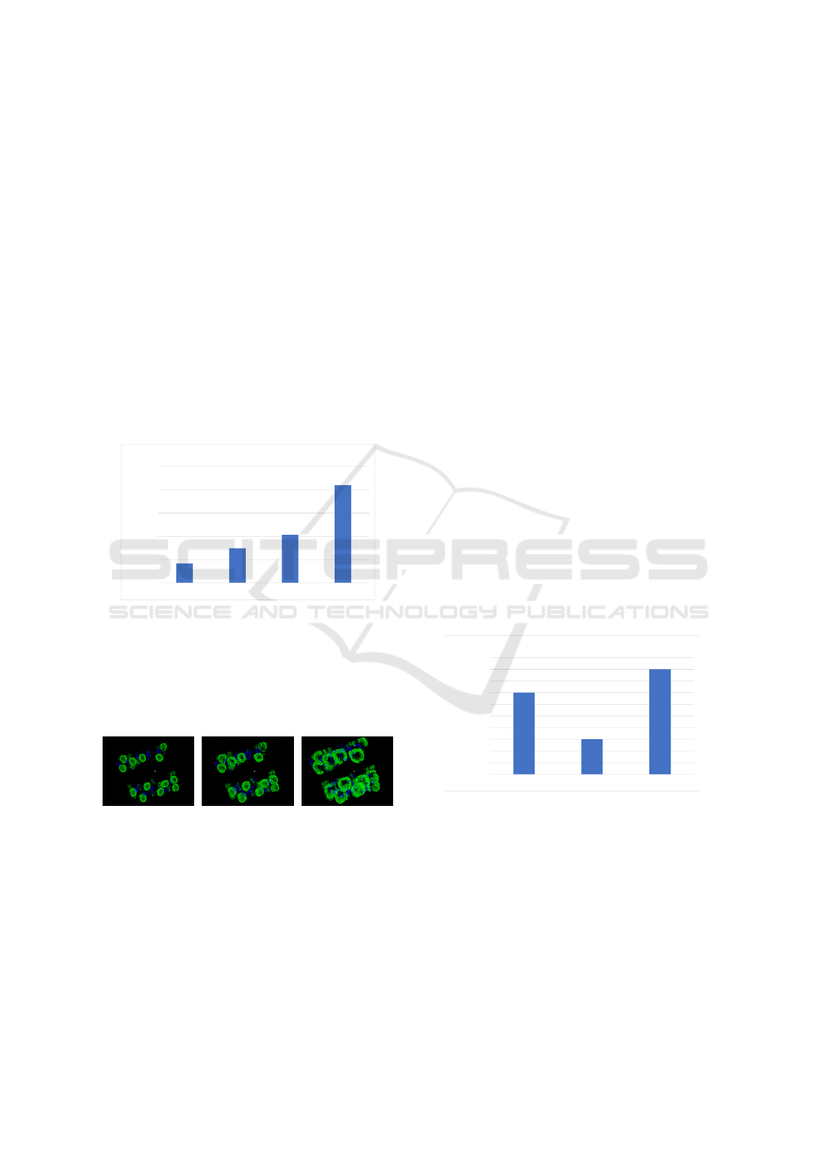
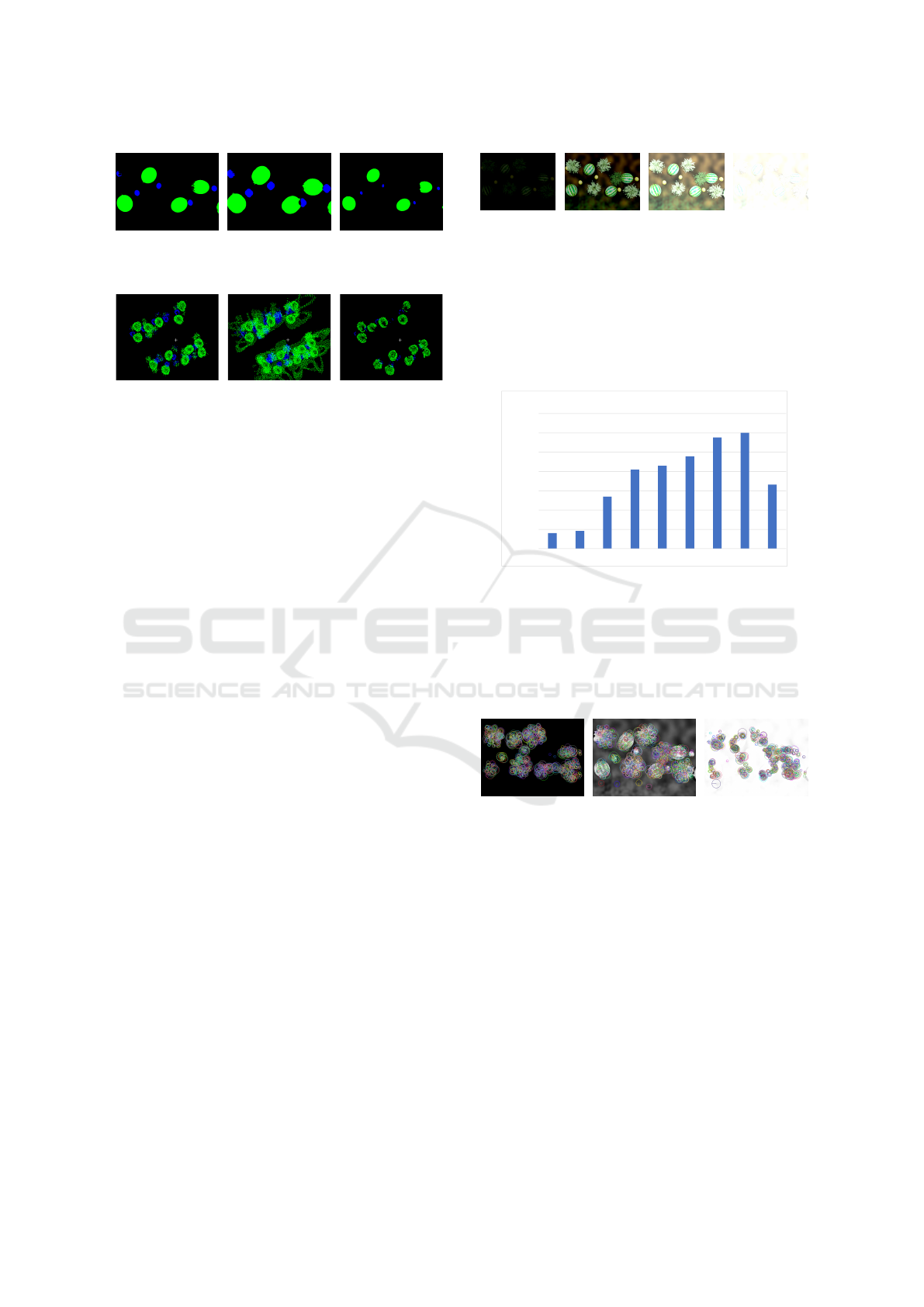
Figure 5 shows the ﬁrst frame of the RGB images,

the depth images and the semantic images obtained

with Vision Blender. In the semantic picture, blue and

green colors represent unripe and ripe watermelons,

respectively. The duck models, which are provided

for free by (Free3D, 2021), are only used in dynamic

scenes and in such cases depicted by a red color.

(a) RGB (b) Depth (c) Semantic

Figure 5: The ﬁrst frame of all RGB, depth and semantic

images (green=ripe, blue=unripe and - not shown in this

static example - red=dynamic objects) in this scene. The

generated data is ideal and used in this work to present a

general method to evaluate SLAM implementations based

on various error models and can be extended to other prob-

lems and research areas which rely on similar data.

All images generated by Blender are perfect and

thus no sensor noise nor distortions caused by seman-

tic segmentation are yet considered.

Compared with the RGB point cloud, the semantic

point cloud can better show the characteristics of the

map, and unnecessary information such as dynamic

objects will not be considered. Therefore, semantic

point clouds will be used for analysis in subsequent

https://github.com/GSORF/Visual-GPS-SLAM

Figure 6: Semantic point cloud generated by

16plants static.

experimental results. Figure 6 shows the semantic

point cloud generated by the data set 16plants static

without additional interference, and its corresponding

ATE is 0.042 m. As we expected, the accuracy of SI-

VSLAM is relatively good when ideal data is used.

3.4 Robustness of SI-VSLAM under the

Inﬂuence of Noise

A Kinect sensor consists of an RGB camera and a ToF

sensor, which are used to obtain RGB pictures and

depth information respectively. The use of sensors

is always associated with random measurement noise

that can be caused by the environment or electrical

devices.

In order to investigate the robustness of the sys-

tem under the inﬂuence of noise, in this experiment

Gaussian noise was added to RGB and depth images

according to the existing literature. The ATE will be

calculated and the generated point cloud will also be

analyzed.

3.4.1 Gaussian Noise in RGB Images

There are many sources of noise in an image which

come from various aspects such as image acquisition,

transmission and compression (Bharati et al., 2021).

There are also many types of noise, such as salt and

pepper noise caused by sudden interference signals,

Gaussian noise caused by sensor heating, or Poisson

noise caused by the particle nature of light. In this

experiment Gaussian noise was taken as an example.

Gaussian noise refers to a type of noise whose

probability density function obeys the Gaussian dis-

tribution

f (x) =

√

2πσ

exp(−

(x −µ)

2σ

). (6)

In equation 6, µ is the expected value and σ is the

standard deviation.

Error Evaluation of Semantic VSLAM Algorithms for Smart Farming

805

Both Gaussian as well as salt and pepper noise are

additive and satisfy

A(x, y) = B(x, y) + H(x, y), (7)

where B(x, y) is the original image at pixel coordi-

nates x and y, H(x, y) is the noise, and A(x, y) is the ﬁ-

nal noisy image. A simple error model is used by sim-

ulating correlated noise via adding the same random

number w ∼ N (µ, σ

) to each color channel. Thus,

Gaussian noise is added to the three-channel RGB im-

age by

(x, y) = b(x, y) + w,

(x, y) = g(x, y) + w,

(x, y) = r(x, y) + w.

(8)

Usually the value of µ is set to zero and σ is the stan-

dard deviation. Figure 7 shows how the ATE changes

in relation to a varying σ.

0.0421

0.0743

0.1035

0.2102

σ = 0 σ = 40 σ = 80 σ = 130

0.05

0.1

0.15

0.2

0.25

ATE (m)

Influence of Gaussian noise (RGB)

Figure 7: Inﬂuence of Gaussian noise in RGB images with

increasing σ.

As depicted in Figure 7, Gaussian noise has a

strong inﬂuence on the robustness of the system. The

higher the σ, the lower the accuracy of the system.

Figure 8 shows the point clouds generated by SI-

VSLAM when σ takes on different values. Interest-

(a) σ = 0 (b) σ = 40 (c) σ = 130

Figure 8: The resulting semantic point clouds with increas-

ing noise in the RGB images.

ingly, the Gaussian noise in the RGB images mainly

distorts the point cloud distribution parallel to the im-

age plane and has no inﬂuence on the depth data of

the point cloud. Therefore, the shape of the distortion

roughly reﬂects the trajectory of the camera.

3.4.2 Gaussian Noise in Depth Images

A Kinect camera uses a ToF-sensor to retrieve the

depth data. In the article Noise Modeling and Un-

certainty Propagation for ToF Sensors (Belhedi et al.,

2012), Amira Belhedi and coworkers took 700 photos

with a ToF sensor at 7 different distances from 0.9m

to 7.4m and came to the conclusion that the depth

noise generated by their ToF sensor can be modelled

by Gaussian noise.

The paper Modeling Kinect Sensor Noise for Im-

proved 3D Reconstruction and Tracking (Nguyen

et al., 2012) found that the depth noise of a Kinect

Sensor can be divided into radial noise (perpendic-

ular to the optical axis, z) and axial noise (parallel to

the z-axis), where the axial noise plays a decisive role,

so the inﬂuence of radial noise can be ignored in the

experiment. The authors pointed out that when the

angle of view of the camera is less than 60

◦

, the depth

noise of the Kinect sensor has the following relation-

ship with the depth value:

(z) = 0.0012 + 0.0019(z −0.4)

, (9)

in other words, the depth noise is only related to the

depth value. With the mathematical model of the

depth noise, noise can be added to the depth image

sequence according to the additive noise model.

In order to clearly show the test results, the case

(z) = 10σ(z) was also simulated in the experiment.

This is an imaginary value, which does not exist in

reality.

0.0421

0.0417

0.0423

σ = 0 σ = σ(z) σ = 10σ(z)

0.0414

0.0415

0.0416

0.0417

0.0418

0.0419

0.042

0.0421

0.0422

0.0423

0.0424

ATE (m)

Influence of Gaussian noise (Depth)

Figure 9: The Gaussian noise of the depth images has no

signiﬁcant inﬂuence on the accuracy of the system (please

note the scale of the chart).

It can be concluded from Figure 9 that the Gaus-

sian noise of the depth image has no inﬂuence on the

accuracy of the system. The reason is that the track-

ing of the pose is achieved through Bundle Adjust-

ment (BA), and the depth data does not participate in

the tracking thread.

The corresponding point clouds in Figure 10 show

that the depth noise affects the distribution of the point

cloud along the Z-axis.

VISAPP 2022 - 17th International Conference on Computer Vision Theory and Applications

806

(a) σ = σ(z, θ) (b) σ = 10σ(z, θ)

Figure 10: The depth of noise inﬂuences the distribution of

the point cloud along the Z-axis.

3.5 Investigation of the Inﬂuences of

Flying Pixels and Missing Depth

Data

Although the RGB-D camera has unlimited perspec-

tives, due to the limitations of the physical hardware

there are still many problems with the depth data in

addition to the noise, e.g. ﬂying pixels and invalid

depth data.

• Flying Pixels: Due to the non-linearity of the im-

age information and the discontinuity of the depth

data, ﬂying pixels can be generated at the edges

of the objects, which theoretically can have any

value between foreground and background (Xiao

et al., 2015).

• Invalid Depth Data: The loss of depth data is an-

other problem with Kinect, usually caused by re-

ﬂections on the surface of smooth objects, translu-

cent objects, or excessive range. Due to the dis-

continuity of the depth data, the depth data is eas-

ily lost at the edges of the objects.

Since these two situations mostly occur on the edge

of the object, both can be simulated using OpenCV’s

canny edge detection algorithm. The extent of the

impact can be adjusted by changing the size of the

extracted edge area. Figure 11 shows the test model

of the ﬂying pixels and the invalid depth data. The

(a) ﬂying pixels (b) invalid depth data

Figure 11: The test model of the ﬂying pixels (random

points in the yellow circle) and the loss of depth value.

results in section 3.4.2 show that the noise and the

changes in the depth images do not affect the accu-

racy and robustness of the system. Therefore the ac-

curacy of the trajectory will not be analyzed in the

experiment. The point clouds in different situations

are shown in Figure 12, where (a) is the original point

cloud, (b) is the point cloud with ﬂying pixels and (c)

is the point cloud with invalid depth data. By com-

(a) Original (b) Flying pixels (c) Invalid depth

Figure 12: The hardware speciﬁc errors using RGB-D cam-

eras result in either additional (b) or missing (c) points.

paring with the original image, it can be seen that

the ﬂying pixels are continuously added to the point

cloud in the form of noise. The impact of ﬂying pix-

els increases as the camera moves and the duration of

measurements increases. In contrast, the loss of depth

data at the edges of the objects has only a very small

inﬂuence on the reconstruction of the point cloud.

The effect of invalid depth values can be reduced by

moving the camera around the objects of interest or

increasing the acquisition time.

3.6 Investigation of the Inﬂuences of

Imprecise Semantic Segmentation

Neural networks are usually used for semantic seg-

mentation in research. However, the number of ob-

jects that a neural network can recognize is often

limited. For example, the PASCAL Visual Object

Classes (VOC) data set (Everingham et al., 2015) con-

sists of 20 objects which is quite coarse. Therefore,

the accuracy of the semantic segmentation is difﬁcult

to guarantee, since misjudgments and unclear object

edges may occur during segmentation.

In addition, video sequences may propagate previ-

ously segmented images by using optical ﬂow meth-

ods. The work of (Zhuang et al., 2021) demonstrates

the challenges around falsely predicted segmentation

masks and presents examples where the object bound-

aries are either dilating or eroding. These two kinds of

distortions can be simulated with OpenCV’s dilating

and eroding operations. From a mathematical point

of view, the principle of dilation and erosion is imple-

mented by convolving an image with a speciﬁc con-

volution kernel. The strength of distortion can be ad-

justed by resizing the convolution kernel using the pa-

rameter s. The larger the value of s, the more serious

the distortion. Figure 13 shows the semantic pictures

when dilation and erosion occurs, respectively. Dur-

ing dilating, the area of the color block increases as

the value of s increases. Eroding is a process oppo-

site to dilating. Figure 14 shows the point cloud when

Error Evaluation of Semantic VSLAM Algorithms for Smart Farming

807

(a) original (b) dilating, s=9 (c) eroding, s=8

Figure 13: Distortion model for semantic segmentation.

(a) original (b) dilating, s=9 (c) eroding, s=8

Figure 14: Point cloud with semantic distortion.

these two distortions occur.

According to Figure 14, dilating has a great in-

ﬂuence on the 3D reconstruction due to the addition

of depth data. Compared with dilating, the damage

to the map by eroding is much smaller. When eroding

occurs, the generated point cloud is always a subset of

the true value. Although eroding causes the absence

of some 3D points, these can be optimized by moving

the camera position or increasing the recording time.

The missing parts are observed again and added to the

3D space.

3.7 Investigation of the System’s

Sensitivity to Light

Compared with laser SLAM, Visual SLAM works

based on the image taken by the camera. Therefore,

Visual SLAM is more sensitive to light, and can’t

even work in places where there is no light or texture.

When analyzing the robustness of a Visual SLAM

system, its sensitivity to light is usually a concern.

According to the ofﬁcial OpenCV documentation,

the brightness and contrast of an image can be ad-

justed by

G(x, y) = αB(x, y) + β, α > 0. (10)

The brightness can be adjusted with β and the con-

trast can be changed with α. Obviously, the change in

contrast also leads to a change in brightness, so that in

this experiment only β will be discussed. The above

equation only holds when the pixel value is not satu-

rated, that is, 0 ≤G(x, y) ≤255. If the value is greater

than 255, it is forced to 255, and if the value is less

than 0, it is set to 0. By increasing or decreasing the

value of β 8 new image sequences were generated.

Figure 15 shows four of the image sequences, where

(a) and (d) have been saturated.

(a) β = -210 (b) β = -60 (c) β = 60 (d) β = 210

Figure 15: Variations of the brightness value β.

According to the trajectory accuracy error at dif-

ferent brightness shown in Figure 16, it can be con-

cluded that when the picture is not saturated, the lower

the brightness, the higher the accuracy of the system.

In general, the system shows good robustness against

changes in brightness.

0.0081

0.0092

0.0270

0.0410

0.0430

0.0478

0.0577

0.0601

0.0332

β=-210

β=-180

β=-120

β=-60

β=0

β=60

β=120

β=180

β=210

0.01

0.02

0.03

0.04

0.05

0.06

0.07

ATE (m)

Comparison of brightness variations

Figure 16: The accuracy of the system under different light-

ing conditions.

If we look at the extraction of feature points when

β = −210, β = 0 and β = 210 (Figure 17), we can

further verify our conclusion. Therefore, the decrease

in brightness is useful for the extraction of feature

points.

(a) β = −210 (b) β = 0 (c) β = 210

Figure 17: The extraction of feature points under different

brightness conditions.

3.8 Investigation of Feature Matching in

Agricultural Scenes

In this section, we will discuss feature matching in the

agricultural environment and the impact of dynamic

objects on the system. For a SLAM system, stable

feature points will become map points and stored in

the map, so the distribution of feature points can be

roughly judged through the sparse point cloud. Fig-

ure 18 is the sparse point cloud generated by Seman-

tic Visual SLAM and the corresponding 3D scene in

Blender. Obviously, feature points on plants are more

likely to generate ﬁnal map points than watermelons.

VISAPP 2022 - 17th International Conference on Computer Vision Theory and Applications

808

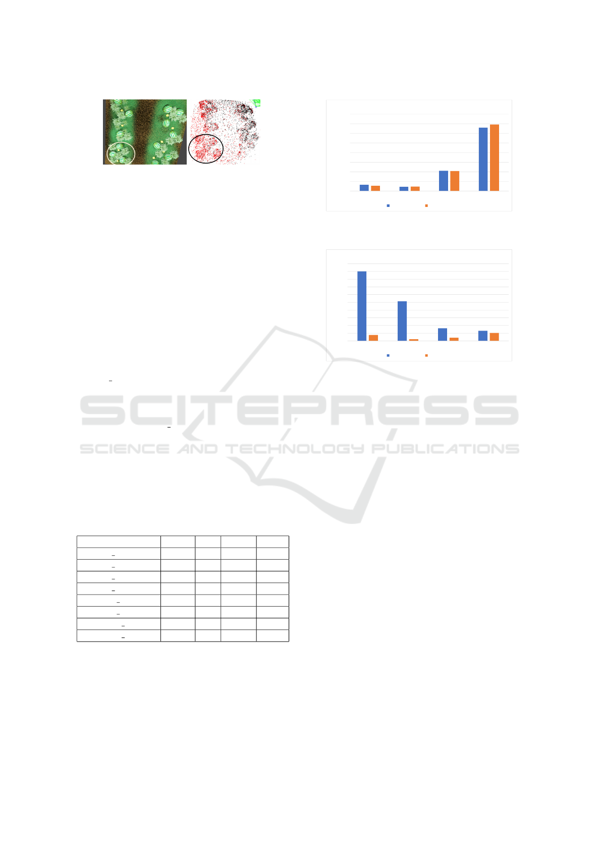
Figure 18: The virtual environment (left) and the recon-

structed sparse point cloud (right). The region in the circle

depicts a more detailed structure, due to stronger image gra-

dients which are used for feature detection and matching.

In other words, plants will generate feature points

with a better quality due to their characteristic image

gradients.

Based on this fact, several hypotheses can be pro-

posed:

1. Providing more high-quality corner patches in the

agricultural scene will lead to a better ATE

2. An increased number of high-quality corners will

increase the robustness of the system against dis-

turbances from dynamic objects

In order to evaluate the ﬁrst hypothesis, three addi-

tional picture sequences are created on the basis of

16plants static. The difference between them is only

the number of plants. In order to assess the second hy-

pothesis, we added 5 ducks to these static agricultural

scenes to generate the corresponding dynamic picture

sequence (i.e. 16plants dynamic). These ducks move

continuously in the scene according to independent

trajectories while the camera is moving in the scene.

The speciﬁcations of new image sequences and

the number of the objects (static plants and dynamic

ducks) are listed in Table 1. The number of watermel-

ons is constant.

Table 1: The data sets used in the experiments and their

properties.

name plants ripe unripe ducks

0plants static 0 13 10 0

0plants dynamic 0 13 10 5

3plants static 3 13 10 0

3plants dynamic 3 13 10 5

16plants static 16 13 10 0

16plants dynamic 16 13 10 5

111plants static 111 13 10 0

111plants dynamic 111 13 10 5

In this experiment, we use SI-VSLAM and ORB-

SLAM2 to test all image sequences (4 static and 4 dy-

namic) respectively. The results are shown in Figure

19 and Figure 20.

0.0129

0.0088

0.0421

0.1317

0.0108

0.0094

0.0415

0.1382

0plants_static 3plants_static 16plants_static 111plants_static

0.02

0.04

0.06

0.08

0.1

0.12

0.14

0.16

ATE (m)

ATE (m) in static environment

ORB-SLAM2 SI-VSLAM

Figure 19: In a static environment, the accuracy of ORB-

SLAM2 and SI-VSLAM is similar.

0.9021

0.5145

0.1631

0.1305

0.0775

0.0214

0.0409

0.1029

0plants_dynamic 3plants_dynamic 16plants_dynamic 111plants_dynamic

0.1

0.2

0.3

0.4

0.5

0.6

0.7

0.8

0.9

ATE (m)

ATE (m) in dynamic environment

ORB-SLAM2 SI-VSLAM

Figure 20: SI-VSLAM is more robust than ORB-SLAM2

in dynamic environments.

4 CONCLUSION

This paper presents a method for the systematic eval-

uation of a Visual SLAM system, ORB-SLAM2,

which uses semantic segmentation as additional in-

put. It proposes to use semantic information to mask

out moving objects and to generate semantic point

clouds and octomaps accordingly. The evaluation was

focused on trajectory accuracy, mapping errors and

the response of the system when moving objects are

present in the scene. First, our implementation was

compared on the TUM RGB-D benchmark data set.

Second, custom synthetic environments were created

for conducting experiments in a controlled setting. By

using error models on RGB, Depth and Semantic Seg-

mentation data it was demonstrated what type of er-

rors can be expected on the output when the proposed

approach is used.

When there are no dynamic objects in the environ-

ment, SI-VSLAM and ORB-SLAM2 have similar ac-

curacy. The structure of the scene, i.e. identical plants

in our case, has a strong inﬂuence on mismatched fea-

ture points.

When there are dynamic objects in the scene,

SI-VSLAM can use semantic segmentation to ﬁlter

out the dynamic objects. Therefore, SI-VSLAM has

higher accuracy in a dynamic environment. It is worth

Error Evaluation of Semantic VSLAM Algorithms for Smart Farming

809

noting that ORB-SLAM2 got the highest accuracy

in the case of 111plants dynamic. Although ORB-

SLAM2 cannot ﬁlter out dynamic objects, the high-

quality feature points make the system more robust in

dynamic environments.

In order to increase the transparency of our work

and make it reproducible for other researchers, we

will provide the source code of our implementation

after the paper is published at https://github.com/

mjtq-slamlearning/SI-VSLAM.

In future work we plan to deploy and evaluate the

proposed system on a real watermelon ﬁeld by work-

ing together with a local farmer. We will hopefully

have a watermelon detector ready and integrated in

our system until the next picking season.

REFERENCES

Belhedi, A., Bartoli, A., Bourgeois, S., Hamrouni, K., Sayd,

P., and Gay-Bellile, V. (2012). Noise modelling and

uncertainty propagation for TOF sensors. In Fusiello,

A., Murino, V., and Cucchiara, R., editors, Computer

Vision – ECCV 2012. Workshops and Demonstrations,

pages 476–485, Berlin, Heidelberg. Springer Berlin

Heidelberg.

Bharati, S., Khan, T. Z., Podder, P., and Hung, N. Q. (2021).

A Comparative Analysis of Image Denoising Prob-

lem: Noise Models, Denoising Filters and Applica-

tions, pages 49–66. Springer International Publishing,

Cham.

Campos, C., Elvira, R., Rodr

ıguez, J. J. G., M. Mon-

tiel, J. M., and D. Tard

os, J. (2021). ORB-

SLAM3: An accurate open-source library for visual,

visual–inertial, and multimap SLAM. IEEE Transac-

tions on Robotics, pages 1–17.

Cartucho, J., Tukra, S., Li, Y., S. Elson, D., and Giannarou,

S. (2020). Visionblender: A tool to efﬁciently gener-

ate computer vision datasets for robotic surgery. Com-

puter Methods in Biomechanics and Biomedical Engi-

neering: Imaging & Visualization, pages 1–8.

Everingham, M., Eslami, S. A., Van Gool, L., Williams,

C. K., Winn, J., and Zisserman, A. (2015). The pascal

visual object classes challenge: A retrospective. Inter-

national journal of computer vision, 111(1):98–136.

Free3D (2021). Free3D: Bird v1. https://free3d.com/

3d-model/bird-v1--94904.html. Accessed: 2021-11-

27.

Ganchenko, V. and Doudkin, A. (2019). Image semantic

segmentation based on convolutional neural networks

for monitoring agricultural vegetation. In Ablameyko,

S. V., Krasnoproshin, V. V., and Lukashevich, M. M.,

editors, Pattern Recognition and Information Process-

ing, pages 52–63, Cham. Springer International Pub-

lishing.

Heckenkamp, C. (2008). Das magische Auge – Grundla-

gen der Bildverarbeitung: Das PMD Prinzip. Inspect,

pages 25–28.

Kalisz, A., Particke, F., Penk, D., Hiller, M., and Thielecke,

J. (2019). B-SLAM-SIM: A Novel Approach to Eval-

uate the Fusion of Visual SLAM and GPS by Exam-

ple of Direct Sparse Odometry and Blender. In VISI-

GRAPP.

Li, Y. and Vasconcelos, N. (2019). REPAIR: Removing

representation bias by dataset resampling. In 2019

IEEE/CVF Conference on Computer Vision and Pat-

tern Recognition (CVPR), pages 9564–9573.

Mur-Artal, R. and Tard

os, J. D. (2017). ORB-SLAM2:

An open-source SLAM system for monocular, stereo,

and RGB-D cameras. IEEE Transactions on Robotics,

33(5):1255–1262.

Nguyen, C. V., Izadi, S., and Lovell, D. (2012). Model-

ing kinect sensor noise for improved 3D reconstruc-

tion and tracking. In 2012 Second International Con-

ference on 3D Imaging, Modeling, Processing, Visu-

alization Transmission, pages 524–530.

Prokhorov, D., Zhukov, D., Barinova, O., Anton, K., and

Vorontsova, A. (2019). Measuring robustness of Vi-

sual SLAM. In 2019 16th International Conference

on Machine Vision Applications (MVA), pages 1–6.

Sturm, J., Engelhard, N., Endres, F., Burgard, W., and Cre-

mers, D. (2012). A benchmark for the evaluation of

RGB-D SLAM systems. In 2012 IEEE/RSJ Interna-

tional Conference on Intelligent Robots and Systems,

pages 573–580.

Xiao, L., Heide, F., O’Toole, M., Kolb, A., Hullin, M. B.,

Kutulakos, K., and Heidrich, W. (2015). Defocus de-

blurring and superresolution for time-of-ﬂight depth

cameras. In 2015 IEEE Conference on Computer Vi-

sion and Pattern Recognition (CVPR), pages 2376–

2384.

Xuan, Z. and David, F. (2018). Real-time voxel based 3D

semantic mapping with a hand held RGB-D camera.

https://github.com/ﬂoatlazer/semantic slam.

Yu, C., Liu, Z., Liu, X., Xie, F., Yang, Y., Wei, Q., and Qiao,

F. (2018). DS-SLAM: A Semantic Visual SLAM to-

wards dynamic environments. 2018 IEEE/RSJ Inter-

national Conference on Intelligent Robots and Sys-

tems (IROS), pages 1168–1174.

Zhang, Z. and Scaramuzza, D. (2018). A tutorial on quanti-

tative trajectory evaluation for visual(-inertial) odom-

etry. In 2018 IEEE/RSJ International Conference on

Intelligent Robots and Systems (IROS), pages 7244–

7251.

Zhuang, J., Wang, Z., and Wang, B. (2021). Video semantic

segmentation with distortion-aware feature correction.

IEEE Transactions on Circuits and Systems for Video

Technology, 31(8):3128–3139.

VISAPP 2022 - 17th International Conference on Computer Vision Theory and Applications

810