Optimization of Adaptive Cruise Control under Uncertainty
Shangyuan Zhang
1,2 a
, Makhlouf Hadji
1 b
, Abdel Lisser
2 c
and Yacine Mezali
1 d
1
Institut de Recherche Technologique SystemX, 8 Avenue de la Vauve, 91120 Palaiseau, France
2
CentraleSupelec, L2S, Université Paris Saclay, 3 Rue Curie Joliot, 91190, Gif-sur-Yvette, France
Keywords:
Adaptive Cruise Control, Optimization, Stochastic Optimization, Autonomous Vehicle.
Abstract:
With the recent developments of autonomous vehicles, extensive studies have been conducted about Adaptive
Cruise Control (ACC), which is an essential component of advanced driver-assistant systems (ADAS). The
safety assessment must be performed on the ACC system before its commercialization. The validation process
is generally conducted via simulation due to insufficient on-road data and the diversity of driving scenarios.
Our paper aims to develop an optimization-based reference generation model for ACC, which can be used
as a benchmark for assessment and evaluation. The model minimizes the difference between the actual and
reference inter-car distance, while respecting constraints about vehicle dynamics and road regulations. ACC
sensors can be impacted by external factors such as weather and produce inaccurate data. To handle the
uncertainty involved, we also propose a chance-constrained stochastic model to reach results with a high level
of confidence. Our numerical results illustrate that the stochastic model outperforms the deterministic model
on randomly generated driving scenarios.
1 INTRODUCTION
During the past two decades, there has been an
increasing trend towards autonomous driving in
both industry and research, which led to many
technological advances and commercial successes.
Autonomous vehicle applications, e.g., advanced
driver assistance systems (ADAS) are extensively
incorporated into modern cars to enhance safety and
improve driving comfort. The most basic feature of
ADAS is adaptive cruise control (ACC), which has
been the focus of researchers and has been actively
studied.
Since 1966, ACC aims to keep a safe distance
with a leading vehicle by adjusting the vehicle’s speed
and acceleration (Levine and Athans, 1966). This
functionality relies both on sensor information about
the location and the motion of the vehicle ahead and
on a controller to regulate the spacing between the
vehicles. An ACC-equipped vehicle drives at a preset
speed until a leading car is detected by the sensors,
then switches to the distance regulation mode by
activating the ACC controller, which calculates the
a
https://orcid.org/0000-0003-0230-8618
b
https://orcid.org/0000-0003-1048-753X
c
https://orcid.org/0000-0003-1318-6679
d
https://orcid.org/0000-0003-1912-9093
safety distance and controls the operation.
Various approaches are applied to achieve the
objective of designing an ACC that most closely
matches the human expert driving behavior in terms
of maneuvering vehicle speed according to different
driving conditions with respect to traffic regulations
and comfortable driving. These ACC systems
target different objectives and are designed under
different standards. Therefore, we need a thorough
validation process to ensure the safety of those
ACC systems and also assess their performance
before making them commercially available. The
result of the validation and evaluation also allows
us to identify potential areas for improvement by
identifying current weaknesses. Due to the fact
that the real road tests, which are time consuming
and costly, cannot cover a large number of driving
scenarios, we carry out the validation process within
a simulator, which can generate driving scenarios.
The driving scenarios include the motion state of the
vehicles at each sampling time.
As part of functional testing of ADAS, the goal
of the ACC validation is to determine whether the
right decision was made, a critical accident was
avoided, and identify potential flaws. The validation
process begins with our model. In our model,
each driving scenario serves as an input, and the
278
Zhang, S., Hadji, M., Lisser, A. and Mezali, Y.
Optimization of Adaptive Cruise Control under Uncertainty.
DOI: 10.5220/0010820400003117
In Proceedings of the 11th International Conference on Operations Research and Enterprise Systems (ICORES 2022), pages 278-285
ISBN: 978-989-758-548-7; ISSN: 2184-4372
Copyright
c
 2022 by SCITEPRESS – Science and Technology Publications, Lda. All rights reserved

reference commands are calculated by solving an
optimization problem. Then we can analyze the
actual commands by comparing them to our generated
reference commands. This process is illustrated in
Figure 1. Generating reference trajectories is a typical
motion planning problem, and there are many ways
to solve it, including sampling-based methods, graph-
based methods, and optimization-based methods.
Among those methods, the optimization approach fits
our needs well, since we can improve comfort and
security of the vehicle by limiting jerks, acceleration,
speed, and relative position, and reach a reasonable
distance ahead by minimizing the value of an
objective function. Furthermore, this approach gives
us a lot of flexibility in tailoring objectives and
constraints according to various driving scenarios and
requirements. These facts led us to devise an ACC
reference generation model based on optimization.
Driving
Scenario
ADAS
Reference
Generator
Commands
Reference
commands
Sensors
Simulation
Comparison
and
validation
Figure 1: Validation process of ADAS.
As part of an ACC system, various types of
sensors may be employed, such as cameras, lidar,
radar etc. Sensor performance is highly influenced
by a variety of factors, including the maintenance
state and environmental conditions (Rasshofer et al.,
2011). There is an inherent level of inaccuracy
in sensor data which must be accounted for when
computations follow. In order to deal with
sensor uncertainty, we develop a chance constrained
stochastic programming model and compare its
simulation results with the deterministic model.
The main contribution of this paper is to study and
compare deterministic and stochastic optimization
models for ACC reference generation. Using
the optimization framework, we solve a quadratic
programming (QP) problem in order to come-up
with the best command to optimize the distance
between two vehicles while satisfying all the problem
constraints. Moreover, we present a comprehensive
comparison of the results obtained with our generated
driving data that simulates realistic driving scenarios
to demonstrate the benefit of the stochastic models.
The remainder of the paper is organized as
follows. Section II discusses different ACC
algorithms under study. Section III describes our
ACC validation model. In Section III, we present
our numerical experiments and compare our different
approaches. Conclusions are provided in Section IV.
2 LITERATURE REVIEW
ACC has been the subject of numerous studies, from
its system design to its on the ground validation.
Many ACC systems employ optimal control
methods (Chehardoli, 2020; Kim, 2012; Zhu et al.,
2018). However, model predictive control (MPC)
has also gained popularity since 2010 (Takahama and
Akasaka, 2018; Li et al., 2010; Naus et al., 2010). A
wide variety of papers has studied ACC from multiple
perspectives, including driving modeling (Seppelt
and Lee, 2015), energy-optimized driving models
(Weißmann et al., 2018), string stability (Liang and
Peng, 1999), and collision avoidance (Lunze, 2018).
Validating the functionality of autonomous
driving is also an important task, not only for ACC
but also other modules which need assessments. In
(Lattarulo et al., 2017), the authors present a global
framework of testing methodology for the evaluation
of path planning and control algorithms, including
a unified test architecture and validation process.
Other similar works include (Lattarulo et al., 2018) ,
(Alnaser et al., 2019).
Aside from the overall testing framework,
individual functionality like ACC should also be
carefully examined. In (Mehra et al., 2015), an
experimental platform is presented for the validation
and demonstration of an optimization-based ACC
controller whilst (Djoudi et al., 2020) present a
simulation based tool chain for reference generation
and test analysis. Several other insightful works on
testing and validating adaptive cruise control can be
found in (Schmied et al., 2015; Shakouri et al., 2015).
3 PROBLEM FORMULATION
3.1 Overview
In this section, we describe the modeling of the
ACC driving scenario and the formulation of the
related optimization problem. A typical ACC driving
scenario includes two cars driving simultaneously in
a single lane, namely, the ego car and the target car.
The ego car is equipped with an ACC system whilst
the target car is the leading car positioned ahead.
Figure 2 illustrates the driving scenario, as well as
the states of two cars at moment t
i
. The purpose
Optimization of Adaptive Cruise Control under Uncertainty
279

of our ACC reference generation is to generate a
sequence of acceleration commands, i.e., the decision
variables in our optimization problem. The objective
of the ego car is to keep a distance from the target
car with respect to different constraints, e.g., vehicle
dynamics, driving comfort, and road regulations.
Figure 2: ACC driving scenario at moment t
i
.
Suppose that the total duration of a driving
scenario is T s composed of n sampling time dt,
i.e. T = ndt with a corresponding timestamp
[t
0
,t
1
,...t
i
,.. . t
n
] where t
i+1
= t
i
+ dt, ∀i ∈
{0,1,. .. n − 1}. At each moment t
i
, the ACC
of the ego car uses sensors to gather the information
from the target car and generates the acceleration
commands. In the following, we list the parameters
and the decision variable used in our model. The
input parameters are given by the ego car sensors,
and the decision variable represents the ACC optimal
commands. The parameters of the ego car are the
initial position x
ego
t
0
, the initial velocity v
ego
t
0
whilst
the parameters of the target car is composed of
the position vector X
tgt
T
= (x
tgt
t
1
,x
tgt
t
2
,.. . x
tgt
t
n
)
T
, the
velocity vector V
tgt
T
= (v
tgt
t
0
,v
tgt
t
1
,.. . v
tgt
t
n−1
)
T
and the
acceleration vector A
tgt
T
= (a
tgt
t
0
,a
tgt
t
1
,.. . a
tgt
t
n−1
)
T
in
the whole driving scenario. The decision variables
is the ACC ego car acceleration commands vector
A
ego
T
= (a
ego
t
0
,a
ego
t
1
,.. . a
ego
t
n−1
)
T
.
Given the decision variable and the initial state of
the ego car, we can derive the velocity and the position
of the ego car by the the equations of motion. The ego
car velocity v
ego
t
i+1
at time t
i+1
is given by the velocity
at the previous sample time v
ego
t
i
and the acceleration
a
ego
t
i
:
v
ego
t
i+1
= v
ego
t
i
+ a
ego
t
i
dt. (1)
The velocity for the whole driving scenario can be
written in matrix form as
V
ego
T
=








v
ego
t
0
.
.
.
v
ego
t
i
.
.
.
v
ego
t
n−1








=








v
ego
t
0
.
.
.
v
ego
t
0
+
∑
k=i−1
k=0
a
ego
t
k
dt
.
.
.
v
ego
t
0
+
∑
k=n−2
k=0
a
ego
t
k
dt








= dtK
n
A
ego
T
+ v
ego
t
0
1
n
,
(2)
where K
n
∈ R
n×n
and 1
n
∈ R
n×1
K
n
=








0 0 0 ... 0 0
1 0 0 ... 0 0
1 1 0 ... 0 0
.
.
.
.
.
.
.
.
.
1 1 1 ... 0 0
1 1 1 ... 1 0








(3)
1
n
=




1
1
.
.
.
1




. (4)
Similarly, the ego car position at time t
i+1
is given
by
x
ego
t
i+1
= x
ego
t
i
+ v
ego
t
i
dt +
1
2
a
ego
t
i
dt
2
. (5)
The corresponding matrix format for all time steps is
X
ego
T
=








x
ego
t
1
.
.
.
x
ego
t
i
.
.
.
x
ego
t
n








=








x
ego
t
0
+ v
ego
t
0
dt +
1
2
a
ego
t
0
dt
2
.
.
.
x
ego
t
0
+
∑
k=i−1
k=0
v
ego
t
k
dt +
1
2
∑
k=i−1
k=0
a
ego
t
k
dt
2
.
.
.
x
ego
t
0
+
∑
k=n−1
k=0
v
ego
t
k
dt +
1
2
∑
k=n−1
k=0
a
ego
t
k
dt
2








= dtM
n
V
ego
T
+
1
2
dt
2
M
n
A
ego
T
+ x
ego
t
0
1
n
,
(6)
where M
n
∈ R
n×n
,
M
n
=






1 0 0 ... 0
1 1 0 ... 0
1 1 1 ... 0
.
.
.
.
.
.
.
.
.
1 1 1 ... 1






. (7)
We use Equation (2) to rewrite Equation (6) in
terms of the initial position, the initial velocity and
the acceleration vector, i.e.,
X
ego
T
= dtM
n
V
ego
T
+
1
2
dt
2
M
n
A
ego
T
+ x
ego
t
0
1
n
= dtM
n
(dtK
n
A
ego
T
+ v
ego
t
0
1
n
)
+
1
2
dt
2
M
n
A
ego
T
+ x
ego
t
0
1
n
= dt
2
(B
n
+
1
2
M
n
)A
ego
T
+ v
ego
t
0
dtC
n
+ x
ego
t
0
1
n
,
(8)
ICORES 2022 - 11th International Conference on Operations Research and Enterprise Systems
280

where B
n
= M
n
·K
n
∈ R
n×n
and C
n
= M
n
·1
n
∈ R
n×1
.
These parameters are summarized in Table 1.
In the following, we use the position and the
velocity vector of the ego car to formulate our
optimization problem.
3.2 Mathematical Modeling
In the following we outline how the generation of
the ACC reference can be viewed as an optimization
problem.
min
A
ego
T
||Q A
ego
T
+ P|| (9)
s.t. dt
2
(B
n
+
1
2
M
n
)A
ego
T
≤ X
tgt
T
− v
ego
t
0
dtC
n
− (x
ego
t
0
+ d
s
)1
n
, (10)
− (v
max
+ v
ego
t
0
)1
n
≤ dtK
n
A
ego
T
≤ (v
max
− v
ego
t
0
)1
n
, (11)
− a
max
1
n
≤ A
ego
T
≤ a
max
1
n
, (12)
− j
max
dt1
n
≤ D
n
A
ego
T
≤ j
max
dt1
n
. (13)
The following part explains in detail how we
derive the objective function (9) and how constraints
(10, 11, 12, 13) are developed.
The objective of ACC is to maintain a safe
distance between the ego car and the target car. In
order to calculate the reference distance between the
ego car and the target car, we define two terms: the
inter-vehicle time tc (e.g., 3 seconds) for the ego
car to brake safely, and the standstill distance δS to
ensure there is always enough room between the two
adjacent cars.
At each moment t
k
, the reference distance of ACC
in platoons is defined by
d
re f
t
k
= (v
ego
t
k−1
− v
tgt
t
k−1
)tc +
1
2
(a
ego
t
k−1
− a
tgt
t
k−1
)tc
2
+ δS.
(14)
So the reference distance vector in the whole
driving scenario is :
D
re f
T
= tc(dtK
n
A
ego
T
+ v
ego
t
0
1
n
−V
tgt
T
)
+
1
2
tc
2
(A
ego
T
− A
tgt
T
) + δS1
n
= (dt · tcK
n
+
1
2
tc
2
I)A
ego
T
−tcV
tgt
T
−
1
2
tc
2
A
tgt
T
+ (δS + v
ego
t
0
tc)1
n
.
(15)
Moreover, the current distance between the ego
car and target car is
D
vehicle
T
= X
tgt
T
− X
ego
T
= X
tgt
T
− [dt
2
(B
n
+
1
2
M
n
)A
ego
T
+ v
ego
t
0
dtC
n
+ x
ego
t
0
1
n
].
(16)
By combining (16) and (15), we obtain the
objective function (9):
min
A
ego
T
||D
vehicle
T
− D
re f
T
||
= min
A
ego
T
||X
tgt
T
− [dt
2
(B
n
+
1
2
M
n
)A
ego
T
+ v
ego
t
0
dtC
n
+ x
ego
t
0
1
n
] − [(dt ·tcK
n
+
1
2
tc
2
I)A
ego
T
−tcV
tgt
T
−
1
2
tc
2
A
tgt
T
+ (δS + v
ego
t
0
tc)1
n
]||
= min
A
ego
T
|| − (dt
2
B
n
+
1
2
dt
2
M
n
+ dt · tcK
n
+
1
2
tc
2
I)A
ego
T
+ X
tgt
T
+tcV
tgt
T
+
1
2
tc
2
A
tgt
T
− δS1
n
− v
ego
t
0
tc1
n
− x
ego
t
0
1
n
− v
ego
t
0
dtC
n
||
= min
A
ego
T
||Q A
ego
T
+ P||,
(17)
where Q = −(dt
2
B
n
+
1
2
dt
2
M
n
+ dt · tcK
n
+
1
2
tc
2
I),
P = X
tgt
T
+ tcV
tgt
T
+
1
2
tc
2
A
tgt
T
− δS1
n
− v
ego
t
0
tc1
n
−
x
ego
t
0
1
n
− v
ego
t
0
dtC
n
and || · || is Euclidean norm.
In addition to the objective function (9), we
describe the following constraints
• Constraint (10) is the minimum distance
constraint which aims to prevent the vehicles
collisions. It is results from
D
vehicle
T
≥ d
s
1
n
. (18)
• Constraint (11) is the maximum velocity
constraint. Routes typically have a maximum
velocity limit which leads to the velocity
constraint. For a given a speed limit v
max
, the
constraint is deduced from
||V
ego
T
||
∞
≤ v
max
. (19)
• Constraint (12) is the maximum acceleration
constraint. Car passengers’ comfort is impacted
by acceleration. Vehicle maneuverings like rapid
acceleration or braking should be avoided. Our
model proposes an acceleration limit of a
max
based on this motivation.
||A
ego
T
||
∞
≤ a
max
. (20)
• Constraint (13) is the maximum jerk constraint.
In jerk, we measure the acceleration variances,
which significantly affect the comfort level of
passengers. A maximum limit j
max
is required for
this constraint.
||J
ego
T
||
∞
≤ j
max
(21)
Optimization of Adaptive Cruise Control under Uncertainty
281

Table 1: Summary of parameters.
Symbols Physical Meaning Relationship
Target Car
A
tgt
T
Acceleration profile during simulation A
tgt
T
= (a
tgt
t
0
,a
tgt
t
1
,.. . a
tgt
t
n−1
)
T
V
tgt
T
Speed profile during simulation V
tgt
T
= (v
tgt
t
0
,v
tgt
t
1
,.. . v
tgt
t
n−1
)
T
X
tgt
T
Position profile during simulation X
tgt
T
= (x
tgt
t
1
,x
tgt
t
2
,.. . x
tgt
t
n
)
T
Ego Car
A
ego
T
Acceleration profile during simulation A
ego
T
= (a
ego
t
0
,a
ego
t
1
,.. . a
ego
t
n−1
)
T
V
ego
T
Speed profile during simulation V
ego
T
= dtK
n
A
ego
T
+ v
ego
t
0
1
n
X
ego
T
Position profile during simulation dt
2
(B
n
+
1
2
M
n
)A
ego
T
+ v
ego
t
0
dtC
n
+ x
ego
t
0
1
n
J
ego
T
Jerk profile during simulation D
n
A
ego
T
Since j
t
i
= (a
ego
t
i
− a
ego
t
i−1
)/d t, the jerk constraint
can be simplified to (13) where D
n
∈ R
n×n
D
n
=








1 0 0 ... 0 0
−1 1 0 .. . 0 0
0 −1 1 ... 0 0
.
.
.
.
.
.
.
.
.
0 0 0 ... 1 0
0 0 0 ... −1 1








. (22)
Given the form of the objective function and
the constraints, our model is a convex quadratic
optimization problem.
In the next section, we will discuss the uncertainty
involved in ACC and how to handle it by stochastic
modeling with chance constraints.
3.3 Stochastic Model
The above presented model is deterministic, i.e., the
input parameters are known in advance. However, in
real life autonomous vehicle problems the parameters
are unknown, and may include different sources of
noise from external factors like weather. Results
are highly dependent upon the quality of input data.
Consequently, the parameters can be better modeled
by random variables, which provides through
probability distributions more robust solutions. In the
following, we model the ACC problem by chance
constrained problem. We suppose that the target
car’s position information x
tgt
t
i
obtained from the ego
car’s sensor include some noise, and follows a normal
distribution x
tgt
t
i
∼ N(µ
i
,σ
2
i
). As a result, X
tgt
T
follows
multivariate normal distribution X
tgt
T
∼ N(µ
T
,Σ
T
),
where
µ
T
=




µ
1
µ
2
.
.
.
µ
n




(23)
and
Σ
T
=





σ
2
1
0 ... 0
0 σ
2
2
... 0
.
.
.
.
.
.
.
.
.
.
.
.
0 0 ... σ
2
n





. (24)
The objective function for this stochastic
optimization problem is
min
A
ego
T
||E(D
vehicle
T
− D
re f
T
)||
= min
A
ego
T
||µ
T
+tcV
tgt
T
+
1
2
tc
2
A
tgt
T
− δS1
n
− v
ego
t
0
tc1
n
− x
ego
t
0
1
n
− v
ego
t
0
dtC
n
− [dt
2
B
n
+
1
2
dt
2
M
n
+ dt · tcK
n
+
1
2
tc
2
]A
ego
T
||
= min
A
ego
T
||Q A
ego
T
+ P
0
||,
(25)
where P
0
= µ
T
+tcV
tgt
T
+
1
2
tc
2
A
tgt
T
−δS1
n
−v
ego
t
0
tc1
n
−
x
ego
t
0
1
n
− v
ego
t
0
dtC
n
.
The minimum distance constraint (18) for each
moment t
i
can be expressed as a chance constraint
(Prékopa, 2013) with a given a threshold α, i.e.,
P(D
vehicle
t
i
≥ d
s
) ≥ α, ∀t
i
= P(x
tgt
i
≥ x
ego
t
i
+ d
s
) ≥ α
= P(
x
tgt
i
− µ
i
σ
i
≥
x
ego
t
i
+ d
s
− µ
i
σ
i
) ≥ α
= F
N
(
x
ego
t
i
+ d
s
− µ
i
σ
i
) ≤ 1 − α
= x
ego
t
i
+ d
s
≤ µ
i
+ σ
i
F
−1
N
(1 − α),
(26)
where F
−1
N
is the quantile function of standard normal
distribution.
For the whole driving scenario, the minimum
distance constraint in a matrix form is
dt
2
(B
n
+
1
2
M
n
)A
ego
T
+ v
ego
t
0
dtC
n
+
(x
ego
t
0
+ d
s
)1
n
≤
ˆ
X
tgt
T
,
(27)
where
ICORES 2022 - 11th International Conference on Operations Research and Enterprise Systems
282

ˆ
X
tgt
T
=





µ
1
+ σ
1
F
−1
N
(1 − α)
µ
2
+ σ
2
F
−1
N
(1 − α)
.
.
.
µ
n
+ σ
n
F
−1
N
(1 − α)





. (28)
Since only the minimum distance constraint is
related to the position of the target car X
tgt
T
, all other
constraints remain unchanged.
4 NUMERICAL EXPERIMENTS
Numerical simulations aim to compare the
deterministic model and stochastic models on
different randomly generated instances. Considering
the sensor error for the ego car, we generate driving
scenarios with different configurations, including the
target car’s trajectory profile and ego car’s initial
state. Next, we formulate the optimization problems
based on the generated parameters and employ a QP
solver to obtain the results (Goldfarb and Idnani,
1983). Finally, we compare the statistical results of
the two models to illustrate the stochastic model’s
effectiveness.
To create an ACC driving scenario, our parameters
consist of two types: the parameters related to the
environment and to the vehicles. The parameters
related to the environment include the simulation
configuration and vehicle regulations, such as the
total scenario duration, velocity limit, collision
avoidance limit, etc. Those parameters reflect the
real life driving rules and simulation setting, therefor
they are fixed during numerical experiments. The
parameters related to the vehicles, such as initial
position, velocity and distance, vary in each randomly
generated instance due to the diversity of driving
scenarios. In order to simulate real driving situations,
the relationship among randomly generated vehicle
parameters should be based on Newton’s laws.
Parameters setup for numerical simulations are
summarized in the sequel:
• Parameters related to the environment
– Total duration of a scenario T : 2s.
– Sampling time step dt: 0.05s.
– Inter-vehicle time tc: 3s.
– Standstill distance σS: 3m.
– Minimum security distance d
s
: 10m.
– Maximum velocity v
max
: 30m/s.
– Maximum acceleration v
max
: 5m/s
2
.
– Maximum jerk j
max
: 5m/s
3
.
– Confidence level α: 0.9.
• Parameters related to the vehicles
– Acceleration of the target car: independent
random variables following a normal
distribution with mean 0 and standard deviation
2, truncated from −5 to 5.
– Initial speed of target car and ego car:
independent random variables following a
normal distribution with mean 15 and standard
deviation 10, truncated from 5 to 25.
– Standard deviation of target car position σ: 1.
– Initial position of target car: random variable
following a normal distribution with mean 200
and standard deviation 1.
– Speed and position of target car: random
variables following normal distributions with
mean calculated by an initial value and the
acceleration vector, and standard deviation 1.
– Initial position of ego car: the initial position
of the target car minus a random variable
following normal distribution with mean 100
and standard deviation 20, truncated from 50
to 150.
As depicted in the previous section, each generated
driving scenario is represented as a QP problem.
There are several methods for dealing with this QP
problem, which can mainly be divided into two
categories: active-set methods and interior point
methods. We use QP solver with Goldfarb–Idnani
algorithm (Goldfarb and Idnani, 1983), which is a
dual active set method, in order to obtain the optimal
solution for our QP problem.
With the configuration above, we generate 100
random driving scenarios, which are then solved by
our QP solver to obtain the results of the deterministic
model and the stochastic model, respectively. Since
the input parameters of the model are based on biased
sensor data, it is possible that the result will violate the
constraints (18) during the driving scenario. Hence,
we measure a model’s performance by examining
its solution’s number of violated constraints. The
more violations of constraints there are, the worse the
solution is.
Amongst 100 test driving scenario cases, we
notice that only 38% of the instances are totally
feasible in view of the deterministic optimal solution
against 56% in view of the stochastic optimal solution
with confidence level α = 0.9.
For an in-depth analysis of constraint violations
across 100 test driving scenarios, Figure 3 visualizes
the constraint violation value d
s
− D
vehicle
T
1
n
, adapted
from constraint (18), for the whole results of the
two models. Figures 3 (a) and 3 (b) show the
constraint violation value for the whole constraints
whilst Figures 3 (c) and (d) show a zoom-in on a
Optimization of Adaptive Cruise Control under Uncertainty
283

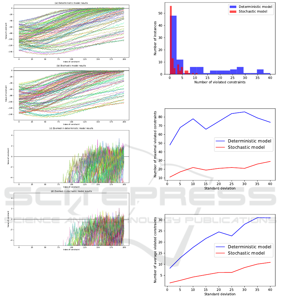
Figure 3: Constraint function values of all instances for
deterministic and stochastic models.
subset of constraints for a better readability. In Figure
3, each curve in its own color displays the constraint
violation values of a driving scenario result, and the
x-axis represents the index of constraints. If the
value at constraint index i exceeds 0, it means that
d
s
> D
vehicle
t
i
, i.e. the constraint (18) is violated at
this sampling time. Figure 3 clearly indicates that the
stochastic model produces fewer violations than the
deterministic one.
Following the visualization of the result, we also
conduct a statistical analysis of the distribution of the
violated constraints number in Figure 4. We observe
that the stochastic model not only produces more
totally feasible solutions with 0 violations, but also
yields fewer violations for cases where the solution is
unfeasible.
Furthermore, keeping all other parameters
Figure 4: Histogram and cumulative histogram of number
of violated constraints for two models.
Figure 5: Maximal violated constraints under different
standard deviation.
Figure 6: Average violated constraints under different
standard deviation.
unchanged, we vary the standard deviation of the
target car position, which depends on sensor’s
precision, from 1 to 40 to compare the performances
of each model. The value of the standard deviation is
gradually increased. We consider 100 tests for each
value, and count the maximal and mean constraint
violations for each model. As shown in Figure 5 and
Figure 6, the stochastic model always outperforms
the deterministic model by producing less constraint
violations.
ICORES 2022 - 11th International Conference on Operations Research and Enterprise Systems
284

5 CONCLUSION AND FUTURE
WORK
We presented in this paper an optimization-based
approach for ACC reference generation taking into
account the uncertainty associated with sensors
information. As a benchmark for ACC system
decision making, our optimization approach can
generate a reference that meets the needs of safety,
comfort, and effectiveness. According to a statistical
analysis of the simulation results, our chance-
constrained based stochastic model can produce more
robust solutions.
For future work, we propose three open research
challenges that have the merit to be addressed:
development of an increasingly sophisticated vehicle
model, modeling of uncertainty involving dependent
random variables, and formulation of objectives that
involve penalties for undesired behavior. The solution
to those challenges will allow us to build a more
general framework to accommodate different needs
for reference generation problem. Furthermore, we
will use this optimization-based reference generation
framework for other autonomous driving functions,
such as lane keeping assistance (LKA) and collision
avoidance.
REFERENCES
Alnaser, A. J., Akbas, M. I., Sargolzaei, A., and
Razdan, R. (2019). Autonomous vehicles scenario
testing framework and model of computation. SAE
International Journal of Connected and Automated
Vehicles, 2(4).
Chehardoli, H. (2020). Robust optimal control and
identification of adaptive cruise control systems in the
presence of time delay and parameter uncertainties.
Journal of Vibration and Control, 26(17-18):1590–
1601.
Djoudi, A., Coquelin, L., and Regnier, R. (2020).
A simulation-based framework for functional
testing of automated driving controllers. In 2020
IEEE 23rd International Conference on Intelligent
Transportation Systems (ITSC), pages 1–6. IEEE.
Goldfarb, D. and Idnani, A. (1983). A numerically stable
dual method for solving strictly convex quadratic
programs. Mathematical programming, 27(1):1–33.
Kim, S. (2012). Design of the adaptive cruise control
systems: An optimal control approach. PhD thesis,
UC Berkeley.
Lattarulo, R., Heß, D., Matute, J. A., and Perez, J. (2018).
Towards conformant models of automated electric
vehicles. In 2018 IEEE International Conference on
Vehicular Electronics and Safety (ICVES), pages 1–6.
IEEE.
Lattarulo, R., Pérez, J., and Dendaluce, M. (2017).
A complete framework for developing and testing
automated driving controllers. IFAC-PapersOnLine,
50(1):258–263.
Levine, W. and Athans, M. (1966). On the optimal error
regulation of a string of moving vehicles. IEEE
Transactions on Automatic Control, 11(3):355–361.
Li, S., Li, K., Rajamani, R., and Wang, J. (2010).
Model predictive multi-objective vehicular adaptive
cruise control. IEEE Transactions on control systems
technology, 19(3):556–566.
Liang, C.-Y. and Peng, H. (1999). Optimal adaptive cruise
control with guaranteed string stability. Vehicle system
dynamics, 32(4-5):313–330.
Lunze, J. (2018). Adaptive cruise control with guaranteed
collision avoidance. IEEE Transactions on Intelligent
Transportation Systems, 20(5):1897–1907.
Mehra, A., Ma, W.-L., Berg, F., Tabuada, P., Grizzle, J. W.,
and Ames, A. D. (2015). Adaptive cruise control:
Experimental validation of advanced controllers on
scale-model cars. In 2015 American Control
Conference (ACC), pages 1411–1418. IEEE.
Naus, G., Ploeg, J., Van de Molengraft, M., Heemels, W.,
and Steinbuch, M. (2010). Design and implementation
of parameterized adaptive cruise control: An
explicit model predictive control approach. Control
Engineering Practice, 18(8):882–892.
Prékopa, A. (2013). Stochastic programming, volume 324.
Springer Science & Business Media.
Rasshofer, R. H., Spies, M., and Spies, H. (2011).
Influences of weather phenomena on automotive laser
radar systems. Advances in Radio Science, 9(B.
2):49–60.
Schmied, R., Waschl, H., and Del Re, L. (2015). Extension
and experimental validation of fuel efficient predictive
adaptive cruise control. In 2015 American Control
Conference (ACC), pages 4753–4758. IEEE.
Seppelt, B. D. and Lee, J. D. (2015). Modeling driver
response to imperfect vehicle control automation.
Procedia Manufacturing, 3:2621–2628.
Shakouri, P., Czeczot, J., and Ordys, A. (2015). Simulation
validation of three nonlinear model-based controllers
in the adaptive cruise control system. Journal of
Intelligent & Robotic Systems, 80(2):207–229.
Takahama, T. and Akasaka, D. (2018). Model predictive
control approach to design practical adaptive cruise
control for traffic jam. International journal of
automotive engineering, 9(3):99–104.
Weißmann, A., Görges, D., and Lin, X. (2018). Energy-
optimal adaptive cruise control combining model
predictive control and dynamic programming. Control
Engineering Practice, 72:125–137.
Zhu, Y., Zhao, D., and Zhong, Z. (2018). Adaptive optimal
control of heterogeneous cacc system with uncertain
dynamics. IEEE Transactions on Control Systems
Technology, 27(4):1772–1779.
Optimization of Adaptive Cruise Control under Uncertainty
285