Towards Robust Continual Learning using an

Enhanced Tree-CNN

Basile Tousside, Lukas Friedrichsen and J

org Frochte

Bochum University of Applied Science, 42579 Heiligenhaus, Germany

Keywords:

Tree-CNN, Continual Learning, Deep Learning, Hierarchical Classiﬁcation, Robust.

Abstract:

The ability to perform continual learning and the adaption to new tasks without losing the knowledge already

acquired is still a problem that current machine learning models do not address well. This is a drawback, which

needs to be tackled for different reasons. On the one hand, conserving knowledge without keeping all of the

data over all tasks is a rising challenge with laws like the European General Data Protection Regulation. On

the other hand, training models come along with CO

footprint. In the spirit of a Green AI the reuse of trained

models will become more and more important. In this paper we discuss a simple but effective approach based

on a Tree-CNN architecture. It allows knowledge transfer from past task when learning a new task, which

maintains the model compact despite network expansion. Second, it avoids forgetting, i.e., learning new tasks

without forgetting previous tasks. Third, it is cheap to train, to evaluate and requires less memory compared

to a single monolithic model. Experimental results on a subset of the ImageNet dataset comparing different

continual learning methods are presented.

1 INTRODUCTION

Continual learning (CL) is a key characteristic of hu-

man intelligence, which remains a daunting problem

in machine intelligence. It refers to the ability of a

neural network to learn consecutive tasks, crucially,

without forgetting how to perform previously learned

tasks.

Unfortunately, the term continual learning is

sometimes used for a wide range of ideas of learning

continually, incrementally and adaptively. In general,

it means that the predictive model is able to smoothly

update, take into account different tasks and data dis-

tributions, while still being able to keep useful knowl-

edge and skills over time. This broad description can

mean dealing with very different tasks like learning

from a stream of different data distributions or just

reusing neural networks in a context one might refer

to as transfer learning. In this paper we concentrate

on classiﬁcation. We denote F as the feature space

and C as the target space of classes. In this context,

the goal of a CL method is to deal with a sequence of

tasks, each containing a classiﬁcation task T

: F → C

⊃ C

t−1

In other words, the set of classes always grows from

task to task and still contains the old classes as sub-

sets. Training on task t is performed using a dataset

. Therefore, without further modiﬁcation in train-

ing, a naively trained neural network tends to over-

write its current weights, causing a replacement of

knowledge about older tasks with the current tasks.

This phenomenon is known to as the catastrophic for-

getting problem (Goodfellow et al., 2013).

Beyond continual learning we discuss the aspect

of robustness in the sense that not all misclassiﬁ-

cations are equal. If classes belong to hierarchical

structures, some of these classes are more related to

each other than others. It is much more acceptable

to misclassify a bee as wasp than as an elephant. A

lot of tasks can be or even are inherently structured

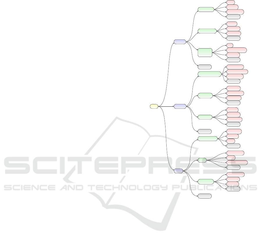
in trees, like the ones in Figure 1 – which will be

used throughout the paper – derived as subset of

ImageNet (Russakovsky et al., 2015). The role

of not here (in Figure 1) is explained later on

and these nodes can be ignored for now. As the

ﬁgure shows, we have trees with different levels

with l ∈ {0, ··· ,3}, where L

is the root-node,

while L

= {animal,arti f act, f ood} is level 1.

Nodes in the deeper levels are denoted as L

2,m

e.g. L

2,0...2

= {vertebrate, invertebrate, domestic

animal}. L

3,n

= {bird, reptile, amphibian} with

n = 0, ... ,2, represents child of vertebrate in the

deepest level L

. This scheme can be extended more

and the extension can also be performed unbalanced.

316

Tousside, B., Friedrichsen, L. and Frochte, J.

Towards Robust Continual Learning using an Enhanced Tree-CNN.

DOI: 10.5220/0010819800003116

In Proceedings of the 14th International Conference on Agents and Artiﬁcial Intelligence (ICAART 2022) - Volume 3, pages 316-325

ISBN: 978-989-758-547-0; ISSN: 2184-433X

In this way, the next task could be just to go deep

regarding birds.

There is a plethora of areas where the application

of such a hierarchical sequential learning comes into

play. Although a traditionally trained neural network

performing joint learning – i.e., accessing all data at

one during training – is in general more promising

in terms of accuracy, this is not always possible or

desired in some real-world scenarios, including but

not limited to:

• Certiﬁcation, e.g. w.r.t. occupational safety in a

smart factory.

• Green AI, along with the accompanying need for

model reuse.

• Data protection and privacy.

Employing machine learning in real life produc-

tion with the risk of human harm or strict quality reg-

ulations - cf. e.g. the ISO 9000 family - comes up

with huge demand regarding rigorous a priori testing

of the model in different settings. Such settings in-

clude additional software solutions around the model

to prevent statistical unlikely but not impossible be-

havior. Smoothly chaining the model such that it is

composed of interlinked, but individually indepen-

dent node partly alleviates this issue by reducing the

size and number of components to be re-evaluated if

a partial change to the database occurs.

The second challenge concerns the aspect of

Green AI (see e.g. (Schwartz et al., 2020)), trying to

prevent unnecessary usage of energy for training pur-

pose. Moreover, in real-world applications like au-

tonomous systems (e.g. autonomous units like robots

or cars), access to computer resources is highly lim-

ited. Hence, restricting the training to necessary level

of new applications is a strongly desired behavior.

In both of the aforementioned scenarios (Certiﬁca-

tion and Green AI), there is always the – although un-

desirable – option to abandon the existing model and

start the training from scratch since the old data are

usually still available. This is however not the case,

when the latter is subject to contemporary privacy and

data protection legislation. One prominent example is

the adoption of the General Data Protection Regula-

tion (GDPR) by the European Union in 2018, which

makes high demands on data protection and privacy

including the requirement to delete data after a given

amount of time. In a similar vein, the California Con-

sumer Privacy Act enacted in 2020 promotes the need

to continually delete consumer processed data over

time.

In such scenarios, it is inherently necessary to in-

crementally build upon the existing model (as done

in our method), since old data are either non-existent

(has been deleted) or not accessible due to privacy

concern, making retraining from scratch practically

unfeasible. In this paper, we propose a novel method

termed as enhanced Tree-CNN to address the contin-

ual learning problem aimed at overcoming the afore-

mentioned problematic.

1.1 Related Work

Previous works addressing continual learning gen-

erally fall under three categories: regularization-

based (Kirkpatrick et al., 2017; Jung et al., 2020),

replay-based (Shin et al., 2017; Riemer et al., 2019)

and architecture-based (Yoon et al., 2018; Li et al.,

2019). Our work belongs to the architecture-based

family and we only discuss this category. The reader

is referred to (Parisi et al., 2019) for an extensive sur-

vey.

Methods in architecture-based family sidestep

catastrophic forgetting by allocating non-overlapping

subsets of model parameters to each task. This is of-

ten achieved by dynamically expending the network

capacity (as in our approach) to handle a new task.

For instance, (Rusu et al., 2016) proposed to expand

the network by augmenting each layer by a ﬁxed num-

ber of neurons for each new task, while keeping the

old layers parameters ﬁxed to avoid forgetting. How-

ever, this method results in a network with excessive

size. (Yoon et al., 2018) proposed to overcome this

limitation by expending each layer with only the nec-

essary number of neurons, but they require several hy-

perparameters and involves cumbersome heuristics to

decide how many neurons to add at each layer. More

recently, (Li et al., 2019) developed a notion of net-

work architecture search to decide, how much to reuse

of the existing network neurons and how much to add.

This method makes the network very compact but is

not effective in term of training time due to the heav-

ily search mechanism.

The publication originating from a different point

of view by (Roy et al., 2020) employs tree-like, dy-

namically growing structures of neural networks. It

contains the basic idea we improve and furthermore

evaluate in our work, thus we discuss the basics

and improvements later on in more details. More-

over, we will show that our approach is scalable and

generic, making it applicable either as a standalone

continual learning method or in combination with a

regularization- or memory-based method.

Towards Robust Continual Learning using an Enhanced Tree-CNN

317

1.2 Contribution

This paper improves and evaluates a tree-like mod-

ular approach for learning sustainable convolutional

neural networks (CNNs) proposed in (Roy et al.,

2020). The improved version can handle an unlim-

ited number of tasks and avoid catastrophic forget-

ting. The main idea is to leverage neural network

modularization via building a tree-CNN in a bottom-

up fashion. This approach enhances continual learn-

ing and robustness. Beyond this, it can help to in-

crease the transparency in the decision-making pro-

cess, therefore it leads to the overall network be-

ing more trustworthy than a single monolithic model.

Another signiﬁcant beneﬁt of this tree-like modular-

ization scheme is the gained robustness of the net-

work with only minor drawbacks in terms of accuracy.

Nevertheless, tree-based approaches come along with

some limitations not discussed in (Roy et al., 2020).

The reason is that in (Roy et al., 2020) CIFAR-100

was used for benchmark problems. The issues mostly

show up in cases with more complex and unbalanced

tasks.

The main contributions of our work are summa-

rized as follows:

• We extend the algorithm from (Roy et al., 2020)

with the option of setbacks.

• We propose a lightweight full prediction approach

for Tree-CNNs.

• We propose a metric to measure errors in tree

structured datasets.

• We propose a subset of ImageNet as real life CL

classiﬁcation benchmark.

• We evaluate the algorithm from (Roy et al., 2020),

our improved version, and EWC (Kirkpatrick

et al., 2017) on this benchmark.

• The latter discussion includes success conditions

for the different approaches.

The paper is organized as follows: Section 2

presents our improvements regarding (Roy et al.,

2020), while in Section 3 we suggest an additional

metric regarding robustness in structured datasets. Fi-

nally, Section 4 includes our suggestion for a bench-

mark problem taken from ImageNet as well as the re-

sults and discussion.

2 ENHANCED TREE-BASED CNN

bird

reptile

amphibian

not here

insect

mollusk

arachnid

not here

cat

working dog

toy dog

not here

instrument

motor vehicle

furnishing

not here

garment

ﬂoor cover

footwear

not here

bridge

housing

memorial

not here

beverage

dessert

dish

not here

edible fruit

seed

unedible fruit

not here

cruciferous

peppers

squash

not here

vertebrate

invertebrate

domestic

animal

not here

instrumentality

covering

structure

not here

alimentation

fruit

vegetable

not here

animal

artifact

food

root

Figure 1: Our proposed subset of the ImageNet Dataset.

Problem Setting. As mentioned earlier, we con-

sider the problem of sequential learning of deep con-

volutional neural network under the scenario, where

an unknown number of tasks with new sets of classes

and an unknown distribution of data are sequentially

provided to the network. Speciﬁcally, our goal is to

train a model for a sequence of tasks, where task t ar-

rives with dataset D

= {x

}

i=1

, such that the ﬁnal

model performs well on the new task as well as on

the previous tasks without considerable performance

loss.

Notations. We denote L

(l ∈ {0, ··· ,3}) as a level

of the tree, where L

and L

are the root and leaf

levels, whereas L

and L

stand for the task-speciﬁc

levels. Beyond this, let K, M be the number of

tasks on level L

and N the number of leaf

nodes or classes in L

. We further denote by T ∈



1,k

}

k=0

,{L

2,m

}

m=0



the set of all tasks in the

ICAART 2022 - 14th International Conference on Agents and Artiﬁcial Intelligence

318

tree. Finally, M

denotes the number of children of

the k

task in L

, whereas N

stands for the number

of children of the m

task in L

Method Overview. Let’s consider a model trained

to tackle task 1, namely to classify images belonging

to K different classes (e.g. animal, artifact, food as in

Figure 1). This model can be viewed as the root node

) of the entire tree-based CNN and its children as

the level 1 (L

) of the hierarchy. Each model in L

is further trained to differentiate between its children,

such that during a prediction, the tree can route sam-

ples to the corresponding next level nodes. The tree

structure is illustrated in Figure 1.

Performing evaluations with this approach, we

found that the root note is very important, because a

misclassiﬁcation performed on its level is inevitable.

If – with a slightly higher probability – artifact has

been chosen incorrectly instead of animal, the predic-

tion will go wrong. This property is even worse, if

one considers continual learning instead of incremen-

tal learning as in (Roy et al., 2020). In incremental

learning, all the data are available to train e.g. the

root node. In the use case of continual learning, it

is possible that a tree-CNN is trained and below the

class bird new sub-classes are introduced. It might be

the case that the root model route the new bird images

correctly into the animal branch. But maybe one of

the new classes is penguin or ostrich. In this case, the

trained convolution layer might end up less efﬁcient.

There are two strategies to make trees-approach – like

(Roy et al., 2020) – capable for continual learning.

One could retrain the root model with a technique,

e.g. EWC (Kirkpatrick et al., 2017), which is capa-

ble to avoid the catastrophic forgetting, or one could

introduce a setback mechanism deeper in the trees.

Of course, it is possible to combine both techniques.

We suggest to start with the introduction of a setback

mechanism and just go for retraining if setbacks are

not capable alone to handle the issue.

In Figure 1, for the setback, new classes not here,

labeled as gray nodes are introduced. These not here

classes are deﬁned by using a given percentage of the

images from one level below. This means e.g. not

here at domestic animals consists of pictures from

the database except domestic animals. Doing so, the

model learns to recognize samples that do not belong

to its position in the hierarchy. This leads to a kind of

open world model, where not here is always the op-

tion that none of the given classes is the correct one,

in the example of domestic animals it is neither a cat,

working- or toy dog.

We observed that the proposed setback mecha-

nism – as brieﬂy described above and more details

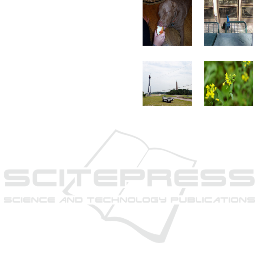
(a) Food - Dog (b) Structure - Bird

Figure 2: Illustration of test samples, which beneﬁted from

the setback mechanisms to be correctly classiﬁed (right la-

bel in each image) after a ﬁrst miss-classiﬁcation (left label

in each image).

in Algorithm 1 – are useful, when it comes to con-

tinual learning. Figure 2 shows four scenarios, where

this mechanism has proven to be effective. In the ﬁrst

scenario (Figure 2a), because of the apple, – the im-

age is ﬁrst classiﬁed incorrectly by the root node as

food. This happened with a very small margin be-

tween the probabilities; animal (0.48), artifact (0.03),

food (0.49). At the food level, the image further gets

classiﬁed as not here. This happens because a portion

of domestic animal images is contained in the not here

category. It follows that the setback mechanism is ac-

tivated and redirects the sample in the tree to L

class

with the next highest probability, i.e., animal, where

the image is ﬁnally classiﬁed correctly as a dog. The

same happen in Figure 2b, 2c, 2d, where the bird, ve-

hicle and seed ﬁrstly got misclassiﬁed as Structure,

Structure and Invertebrate respectively, before being

rescued by the setback mechanism.

Another new feature of our method belongs to the

information provided by the algorithm during predic-

tion. A tree-model built according to (Roy et al.,

2020) – here CIFAR 100 was used – has the same

structure as ours except the not here nodes. During

prediction, the sample is rooted from the root node to

a leaf node of the tree. The routing performed is based

on the highest probability of a class. Algorithm 1 in

section 3.2 of (Roy et al., 2020) returns the selected

class. Following this scheme, any information about

the distribution of the probability along the classes is

lost. Theoretically, one can consider a second mode

for the tree, in which all nodes are used for a pre-

diction, and the probability is calculated along the

Towards Robust Continual Learning using an Enhanced Tree-CNN

319

Algorithm 1: Prediction with Setbacks.

1: Input: X image to predict

2: L

root trained model

3: {L

1,k

}

k=0

level 1 trained tasks

4: {L

2,m

}

m=0

level 2 trained tasks

5: Output: P({L

3,n

}

n=0

) vector of leaf nodes

class probabilities

6: procedure:

7: predict class k using L

(X), save probabilities

and set

k = k

8: setback = False

9: repeat

10: predict class m using L

1,k

(X), save probabili-

ties and set ˜m = m

11: mark L

1,k

as visited

12: while m = not here do

13: mark L

2,m

as visited

14: if all nodes visited in L

then

15: set k =

k and m = ˜m

16: break

17: end if

18: set k to the value of the class with the next

highest probability of L

(X)

19: recalculate probabilities

20: predict class m using L

1,k

(X) and save prob-

abilities

21: mark L

1,k

as visited

22: end while

23: predict class n using L

2,m

(X) and save proba-

bilities

24: mark L

2,m

as visited

25: while n = not here do

26: set m to the value of the class with the next

highest probability of L

1,k

(X)

27: recalculate probabilities

28: mark L

2,m

as visited

29: if m = not here or all children of L

1,k

were

visited then

30: Set k to the value of the class with the next

highest probability of L

(X)

31: setback = True

32: end if

33: predict class n using L

2,m

(X) and save prob-

abilities

34: end while

35: if all of L

2,m

for m = 0,. .., M were visited

then

36: evaluate the tree ignoring all setbacks and

use the highest probabilities ignoring not

here

37: end if

38: until not setback

branches of the tree. Unfortunately, this would come

along with a huge increase of CPU usage during the

prediction. To overcome both limitations (probability

distribution lost and huge CPU usage), we propose a

probability propagation and recalculation mechanism

as described bellow.

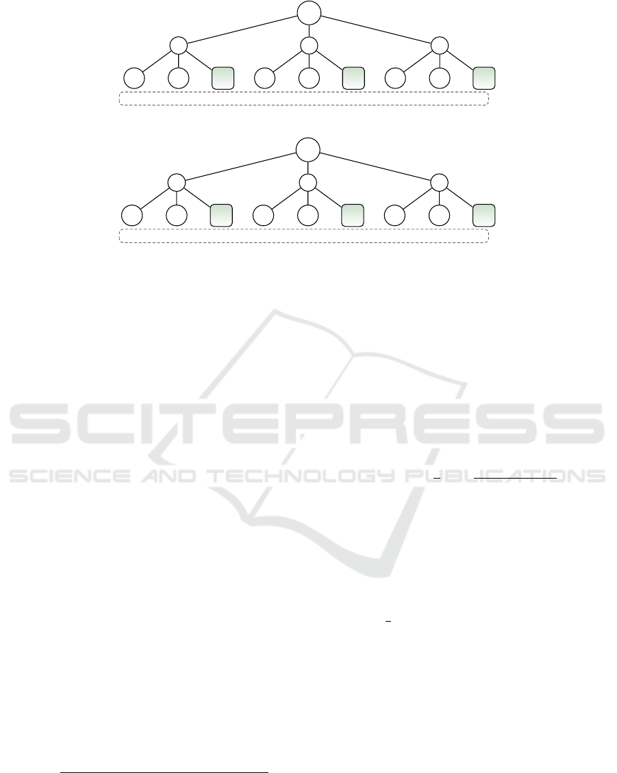
Let’s consider predicting a test image X

, then

O(N, i) = P({L

3,n

}

n=0

) is an output vector contain-

ing the probability of all leaf classes, which is ob-

tained by propagating the probability of each node

in L

and L

to its corresponding leaf node. Fig-

ures 3 and 4 illustrate this mechanism and show how

O(N, i) is calculated. In Figure 3, the root node clas-

siﬁes the test sample as belonging to class B with

a probability of 0.6. At node B, the sample is fur-

ther classiﬁed as belonging to leaf node B

with a

probability of 0.7. The dashed rectangle at the bot-

tom shows the vector O(N,i), containing computed

class probability of each leaf node. While the val-

ues for leaf nodes B

and B

are obvious, the com-

putation of A

and A

probabilities demonstrates the

not here propagation. In fact, σ

= 0.6 × 0.1 prob-

ability is associated to not here in B. This not here

class in B was trained with images of A

nodes. Therefore, we propagate σ

– probability of B

not here – to these nodes and compute their ﬁnal out-

put probabilities as: P(A

) = P(A

) =

0.3

+ σ

and

P(C

) = P(C

) =

0.1

+ σ

with σ

0.6×0.1

being

the propagated probability of B not here shared by

and C

In the case of Figure 4, there are two runs of the

tree showed in red and blue respectively. During the

ﬁrst run, the root node classiﬁes the image incorrectly

as belonging to B. Fortunately, the setback mecha-

nism gets activated at B and routes the image back to

the root level. Now we choose to handle this decision

as B is impossible statement. Thus, the probability of

B is zeroed and equally distributed through A and C.

Then the class with the next highest probability (dur-

ing ﬁrst run) gets selected, which is A. The probability

ﬂowing to A is then computed as the probability of A

at the ﬁrst run added to the distributed probability of

B (at ﬁrst run), i.e., P(A) = 0.4 +

0.5

. At A, the image

is further classiﬁed as belonging to A

with a prob-

ability of 0.7. The not here class at A is predicted

with a probability of 0.2, which is then distributed

through A1 and A2. The ﬁnal probability of A

and A

is then computed as P(A

) =



0.7 +

0.2



× 0.65 and

P(A

) =



0.1 +

0.2



× 0.65 respectively. The prob-

ability P(C

) and P(C

) are computed via a similar

strategy, which lead the three levels tree from the

example of Figure 4 to the Output vector O(N,i) =

[0.52, 0.13, 0, 0, 0.175, 0.175].

ICAART 2022 - 14th International Conference on Agents and Artiﬁcial Intelligence

320

root

not

here

not

here

not

here

0.3

0.3/2

0.6

0.7

0.2

0.1

0.1/2

0.165 0.165 0.6 × 0.7 0.6 × 0.2 0.065 0.065

Figure 3: Tree demonstrating the computation of leaf node probability vector in one shot.

root

not

here

not

here

not

here

0.4 — 0.4 + 0.5/2 = 0.65

0.7

0.1

0.2

0.5 — 0.0

0.1

0.8

0.1 — 0.1 + 0.5/2 = 0.35

0.35/2

0.52

0.13 0.0 0.0

0.175 0.175

Figure 4: Tree demonstrating the computation of leaf node probability vector in two runs.

The behavior described above is denoted as recal-

culate probabilities in Algorithm 1. It goes along with

the not here mechanisms, making them powerful tools

for tree-CNNs as will be validated in the experiment

section.

3 ADAPTING A NORM FOR

ROBUST SEMANTIC

PREDICTION

While it can be taken for granted, that through explicit

structural deﬁnition and the availability of interim re-

sults, modularization in form of tree-CNNs simpli-

ﬁes interpretability and facilitates error traceability,

the implications of the approach on model robustness

or semantic accuracy necessitate further investigation.

The standard accuracy is quite often misleading in

class sets with a semantic distance. To elaborate this

point, consider e. g. the obstacle detection system of

an autonomous vehicle. In this case, it is of less im-

portance for such a system to be able to accurately tell

apart men and woman than it is to reliably distinguish

between humans and e. g. road signs. We denote this

as predictive conceptual proximity and discuss below,

how to measure it by an appropriate norm.

We ﬁrst measure the semantic accuracy at each

level by modifying the semantic distance – a metric

– as deﬁned by (Fergus et al., 2010).

i, j

intersect(path(i), path( j))

max(length(path(i)), length(path( j)))

In the deﬁnition taken from (Fergus et al., 2010) the

semantic distance S

i, j

between classes i and j – which

are leaves in the tree – is deﬁned as the number of

nodes shared by their two parent branches, divided by

the length of the longest of the two branches. There-

fore, path(i) is the path from the root node to the i-

th node in a hierarchical label structure given by the

nodes, whereas intersect gives the number of shared

nodes. Thus, we have 0 < S

i, j

≤ 1, with 1 in case of

an identical object and 0 as lower limit for two com-

pletely different objects.

Taking this as an initial concept, we now use

this semantic distance as weight factor for errors per-

formed by a model on a test set D = {(x

)| i =

1,. .., I} to deﬁne the semantic accuracy

(sac

sac

∑

k=1



,M(x

)

− S

min

1 − S

min



with S

min

= min

i, j

(1)

If a model is 100% accurate, then the

semantic accuracy

(sac

) and the common accuracy

are both 1. In any other case the semantic accuracy

will provide a more detailed description how robust

the prediction is. In the example shown in Figure

1, S

min

. Thus, the transformation leads again

to the fact that a model, which would always pre-

dict the maximum distance class, will achieve a

semantic accuracy

of zero. Like for the common

p-norms, the value of p smooths or sharps the

measurement. With this semantic accuracy

we now

have a tool to compare different models regarding

their robustness.

4 EXPERIMENTS AND ANALYSIS

In this section, we demonstrate the beneﬁts of our

method on hierarchical image classiﬁcation datasets

in a continual learning setup.

Towards Robust Continual Learning using an Enhanced Tree-CNN

321

4.1 Dataset and Baselines

Some problems arise, when a dataset is unbalanced

and comes along with a descent size. Consequently,

many challenges can not be recognized in practice on

datasets like CIFAR100 or MNIST. Hence, we con-

duct experiments on a split of the popular ImageNet,

which is a more challenging and real world related

datasets in comparison to common CL benchmarks

like CIFAR or MNIST. Our split of ImageNet is gen-

erated as shown in Figure 1, representing 152 GB of

images, which leads to a three level hierarchy consist-

ing of twelve tasks presented to the CL models in the

alphabetical order. Each class in level 3 (represented

in red) – except the not here class – contain data of

all its child classes in the ImageNet hierarchy. The

resulting database is therefore unbalanced and con-

tains for example more images regarding animals than

food.

We compare our method against different base-

lines; ﬁrst of all the elastic weight consolidation

(EWC) (Kirkpatrick et al., 2017), which is a standard

comparative baseline in CL research. The second

baseline we compare with is the original tree-based

incremental learning approach (Roy et al., 2020),

which uses CIFAR as dataset. Beyond this, we pro-

vide an – in a way – upper-bound model, which learns

on all the tasks jointly, that is by accessing training

data at once in a traditional way. We refer to this

model as the monolithic model.

4.2 Model and Training

The starting point for our models are NASNetMo-

bile (Zoph et al., 2018) and NASNetLarge (Zoph

et al., 2018). For both, we start with the weights

trained on the whole ImageNet and adjust them on

our sub-set of ImageNet. The EWC CL model in our

setup is built by applying EWC to the NASNetLarge

architecture with some modiﬁcations mentioned later

on. The monolithic model as well is trained using

the NASNetLarge network. For both tree-CNNs each

of the 13 nodes contains a NASNetMobile version,

which is trained for 15 epochs using a batch size of

256.

In summary, there are four big models, two based

on NASNetLarge (EWC and monolithic) and two

based on 13 NASNetMobile (original Tree-CNN and

eTree-CNN). Table 2 indicates, that the full tree with

13 models of the size of NASNetMobile has still

fewer degrees of freedom than the NASNetLarge net-

work, which makes it cheaper to train and memory

efﬁciently.

One aspect regrading the tree-CNN approaches,

which is worth mentioning, is the fact that in higher

levels the number of training examples shrink. There-

fore, training these nodes relies more on reusing the

weights from the next abstract level and carefully

choosing optimisation parameters like the learning

rate. Otherwise, one may face some kind of overﬁt-

ting.

4.3 Evaluation

We use two metrics to evaluate continual learning al-

gorithms in hierarchical datasets. The ﬁrst one is the

all-important average classiﬁcation accuracy as de-

ﬁned in (Chaudhry et al., 2018). More speciﬁcally,

after training on task t the reported accuracy is the av-

erage accuracy obtained from testing on task 1,...,t.

The second metric is the semantic accuracy as deﬁned

in Section 3.

4.4 Results and Analysis

Table 1 reports the accuracy of all four methods in

different ﬂavors. The ﬁrst and second level accuracy

presents the average classiﬁcation accuracy – as de-

ﬁned in Section 4.3 – after training on L

and L

tasks respectively. The accuracy on L

outlines a sim-

ilar effect, however, since it is the last level in the

hierarchy, it represents the same value as the overall

model accuracy as such. In papers dealing with Ima-

geNet, this is often denoted as Top-1-Accuracy. The

last row of Table 1 provides results for the semantic

accuracy deﬁned in Section 3. Moreover, the last col-

umn shows results for the monolithic model, which is

trained without the need of CL, therefore accessing all

training data at once. We use this as an upper-bound

reference model and provide percentage values for all

other models compared to this one.

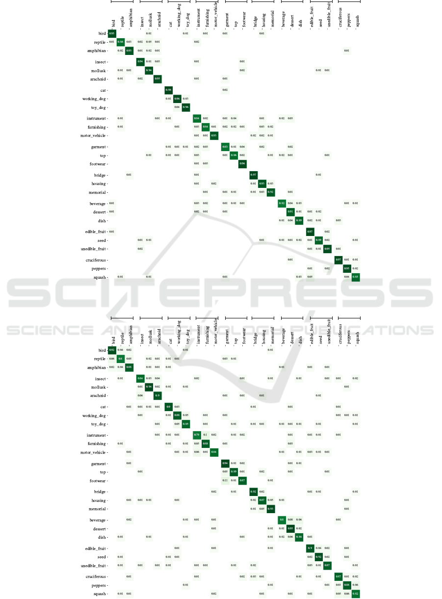
Figures 5 and 6 visualize the confusion matrices

for enhanced Tree-CNN (eTree-CNN) and the EWC

approach after training on all tasks. They provide fur-

ther insides on how the misclassiﬁcations are ﬁnally

distributed. Overall, the results indicate that all CL

methods were capable to learn the multiple ImageNet

tasks in sequence without forgetting. Consistently,

we see that eTree-CNN is able to perform the results

closest to the upper boundary given by the monolithic

model by maintaining high performance on all pre-

viously learned tasks throughout learning later tasks.

Furthermore, we observed that both tree-CNN ap-

proaches perform well regarding their robustness and

semantic accuracy. In general, for all norms, the set-

back approach has proven to be helpful. Interestingly,

as can be seen in Table 1, sac

reﬂects more or less the

ICAART 2022 - 14th International Conference on Agents and Artiﬁcial Intelligence

322

vertebrate invertebrate

domestic

animal

instru-

mentality covering

structure alimentation fruit

vegetable

Figure 5: Results of eTree-CNN displayed in a confusion matrix with sub-sets of the different abstraction levels.

vertebrate invertebrate

domestic

animal

instru-

mentality covering

structure alimentation fruit

vegetable

Figure 6: Results of EWC displayed in a confusion matrix with sub-sets of the different abstraction levels

Towards Robust Continual Learning using an Enhanced Tree-CNN

323

Table 1: Achieved accuracy for different approaches with continual learning (CL) and a completely trained reference value

(without CL).

Norm EWC Tree-CNN Enhanced Tree-CNN Monolithic

with CL with CL with CL without CL

(Level 3) accuracy 0.869 (90.5%) 0.890 (92.7%) 0.917 (95.4%) 0.960 (100%)

Level 2 accuracy 0.898 (92.3%) 0.927 (95.3%) 0.944 (97.0%) 0.973 (100%)

Level 1 accuracy 0.923 (93.5%) 0.952 (96.5%) 0.976 (98.9%) 0.987 (100%)

semantic accuracy

0.637 (79.4%) 0.681 (84.9%) 0.709 (88.4%) 0.802 (100%)

semantic accuracy

0.621 (87.5%) 0.653 (92.0%) 0.670 (94.4%) 0.71 (100%)

Table 2: Total degrees of freedom to be trained for different

models.

Methods Model Total DoF

eTree-CNN NASNetMobile ×13 57.2 Mio

Tree-CNN NASNetMobile ×13 57.2 Mio

EWC NASNetLarge ×1 85.4 Mio

Monolithic NASNetLarge ×1 85.4 Mio

same relative behavior as the common accuracy. On

one hand, it turned out, that higher p values are not

more suitable to measure semantic accuracy than the

common accuracy. On the other hand, lower p (here

sac

) are sensible to measure these changes. Using

this norm, the differences between Tree-CNN, eTree-

CNN and EWC regarding semantic accuracy are bet-

ter emphasized. Over all of these different norms and

derived metrics, one can see the advantage of the tree-

models compared to EWC. While the difference on

level 1 between the reference model and the eTree-

CNN is about 1%, it is more than 6% for the EWC

and over 3% for Tree-CNN. This is even worse for

sac

, which is more sensitive regarding errors per-

formed outside the hierarchy structures. It delivers

about 20%, 15%, 12% difference towards the refer-

ence model and EWC, Tree-CNN and eTree-CNN re-

spectively.

A conclusion that can be taken from Table 1 is

that our eTree-CNN outperforms all baselines signiﬁ-

cantly in terms of average accuracy and semantic dis-

tance, whereas Tree-CNN by (Roy et al., 2020) per-

forms superior to EWC. However, it is worth not-

ing that these superior results for both tree-CNN ap-

proaches come along with a limitation EWC does not

contain. In fact, to use the Tree-CNNs, a dataset ex-

hibiting a hierarchy structure is needed, while EWC

can be applied on any dataset.

Moreover, we can observe in Figure 6 (EWC con-

fusion matrix), that although the errors are mainly

distributed within the level 2 hierarchy, the confu-

sion matrix, however it is less sparse compared to

eTree-CNN shown in Figure 5. This is due to the

fact, that in ImageNet a lot of pictures contain pat-

terns of more than one category, which makes the CL

problem more challenging compared to standard CL

benchmarks like MNIST or CIFAR. Some of such test

samples containing more than one category can be

seen in Figure 2, for example animal and food (2a)

or animal and structure (2b). In such situations, our

setback mechanism as described earlier allows eTree-

CNN to still produce strong results at differentiating

past tasks and current tasks (where structure of past

task might appear).

An empirical conclusion, that can be made out of

this is, that eTree-CNN consistently performs better

than all other methods, partially thanks to the way it

rescues some misclassiﬁcation occurred mostly due to

duplicate structure in the test sample. The idea of em-

powering the model with a setback mechanism along

its recalculated probability tool seems to be working

well with complex data-sets like ImageNet given di-

rections for forthcoming work, where eTree-CNN can

be extended to other real-world applications of CNNs.

5 CONCLUSION

We proposed eTree-CNN, a new tree-based continual

learning method for overcoming catastrophic forget-

ting. A concept of stepbacks was introduced, which

routes back to previous levels when evaluating the

tree, to correct a possible misclassiﬁcation. Using a

suggested benchmark based on ImangeNet, the pro-

posed approach provides higher accuracy and robust-

ness compared to other continual learning methods.

Moreover, it is cheaper to train and consumes much

less memory than monolithic approaches.

ACKNOWLEDGEMENTS

This work was funded by the federal state of North

Rhine-Westphalia and the European Regional Devel-

opment Fund FKZ: ERFE-040021.

ICAART 2022 - 14th International Conference on Agents and Artiﬁcial Intelligence

324

REFERENCES

Chaudhry, A., Dokania, P. K., Ajanthan, T., and Torr, P. H.

(2018). Riemannian walk for incremental learning:

Understanding forgetting and intransigence. In Pro-

ceedings of the European Conference on Computer

Vision (ECCV), pages 532–547.

Fergus, R., Bernal, H., Weiss, Y., and Torralba, A. (2010).

Semantic label sharing for learning with many cate-

gories. In European Conference on Computer Vision,

pages 762–775. Springer.

Goodfellow, I. J., Mirza, M., Xiao, D., Courville, A., and

Bengio, Y. (2013). An empirical investigation of

catastrophic forgetting in gradient-based neural net-

works. arXiv preprint arXiv:1312.6211.

Jung, S., Ahn, H., Cha, S., and Moon, T. (2020). Con-

tinual learning with node-importance based adap-

tive group sparse regularization. arXiv preprint

arXiv:2003.13726.

Kirkpatrick, J., Pascanu, R., Rabinowitz, N., Veness, J.,

Desjardins, G., Rusu, A. A., Milan, K., Quan, J.,

Ramalho, T., Grabska-Barwinska, A., et al. (2017).

Overcoming catastrophic forgetting in neural net-

works. Proceedings of the national academy of sci-

ences, 114(13):3521–3526.

Li, X., Zhou, Y., Wu, T., Socher, R., and Xiong, C. (2019).

Learn to grow: A continual structure learning frame-

work for overcoming catastrophic forgetting. In In-

ternational Conference on Machine Learning, pages

3925–3934. PMLR.

Parisi, G. I., Kemker, R., Part, J. L., Kanan, C., and

Wermter, S. (2019). Continual lifelong learning with

neural networks: A review. Neural Networks, 113:54–

71.

Riemer, M., Klinger, T., Bouneffouf, D., and Franceschini,

M. (2019). Scalable recollections for continual life-

long learning. In Proceedings of the AAAI Conference

on Artiﬁcial Intelligence, volume 33, pages 1352–

1359.

Roy, D., Panda, P., and Roy, K. (2020). Tree-CNN: A hi-

erarchical deep convolutional neural network for in-

cremental learning. Neural networks: the ofﬁcial

journal of the International Neural Network Society,

121:148–160.

Russakovsky, O., Deng, J., Su, H., Krause, J., Satheesh, S.,

Ma, S., Huang, Z., Karpathy, A., Khosla, A., Bern-

stein, M., et al. (2015). Imagenet large scale visual

recognition challenge. International journal of com-

puter vision, 115(3):211–252.

Rusu, A. A., Rabinowitz, N. C., Desjardins, G., Soyer,

H., Kirkpatrick, J., Kavukcuoglu, K., Pascanu, R.,

and Hadsell, R. (2016). Progressive neural networks.

arXiv preprint arXiv:1606.04671.

Schwartz, R., Dodge, J., Smith, N. A., and Etzioni, O.

(2020). Green ai. Communications of the ACM,

63(12):54–63.

Shin, H., Lee, J. K., Kim, J., and Kim, J. (2017). Continual

learning with deep generative replay. arXiv preprint

arXiv:1705.08690.

Yoon, J., Yang, E., Lee, J., and Hwang, S. J. (2018). Life-

long learning with dynamically expandable networks.

ICLR.

Zoph, B., Vasudevan, V., Shlens, J., and Le, Q. V. (2018).

Learning transferable architectures for scalable image

recognition. In Proceedings of the IEEE conference on

computer vision and pattern recognition, pages 8697–

8710.

Towards Robust Continual Learning using an Enhanced Tree-CNN

325