Post-hoc Global Explanation using Hypersphere Sets
Kohei Asano and Jinhee Chun
Graduate School of Information Sciences, Tohoku University, Sendai, Japan
Keywords:
Explanations, Interpretability, Transparency.
Abstract:
We propose a novel global explanation method for a pre-trained machine learning model. Generally, machine
learning models behave as a black box. Therefore, developing a tool that reveals a model’s behavior is impor-
tant. Some studies have addressed this issue by approximating a black-box model with another interpretable
model. Although such a model summarizes a complex model, it sometimes provides incorrect explanations
because of a gap between the complex model. We define hypersphere sets of two types that respectively
approximate a model based on recall and precision metrics. A high-recall set of hyperspheres provides a
summary of a black-box model. A high-precision one describes the model’s behavior precisely. We demon-
strate from experimentation that the proposed method provides a global explanation for an arbitrary black-box
model. Especially, it improves recall and precision metrics better than earlier methods.
1 INTRODUCTION
Machine learning models are applied to various tasks
to produce highly accurate predictions. Users face an
interpretability issue: machine learning models have
difficulty elucidating black-box model behavior be-
cause these models tend to be complex and tend to
lack readability. Interpretability issues present ur-
gent difficulties to be resolved in the machine learning
field. Especially, interpretability is important when
applied to sensitive fields such as credit risks(Rudin
and Shaposhnik, 2019), educations(Lakkaraju et al.,
2015), and health care(Caruana et al., 2015).
Many studies have been conducted recently to im-
prove machine learning model transparency(Guidotti
et al., 2018b; Roscher et al., 2020; Pedreschi
et al., 2019). There is an aspect of an explana-
tion method that presents local and global scopes
of interpretability. A local explanation provides
a feature effect(Lundberg and Lee, 2017) or local
decision rule(Guidotti et al., 2018b; Asano et al.,
2019; Asano. and Chun., 2021) for individual
predictions. Conversely, a global explanation re-
flects the overall model’s behavior. Users can eval-
uate the model reliability. Several global expla-
nation approaches exist, such as those elucidating
feature importance(Lundberg et al., 2020) or ef-
ficiency(Friedman, 2001; Zhao and Hastie, 2021)
and building a surrogate model(Breiman and Shang,
1996; Hara and Hayashi, 2018). Among the ap-
proaches are methods that build another explanatory
model approximating a pre-trained model ex-post.
Such methods are called post-hoc explanations.
We propose a novel post-hoc and model-agnostic
global explanation method using surrogate models.
We consider that an issue for further improvement
is the consistency of an explanation. With an ear-
lier global surrogate methods, they approximate a pre-
trained black-box model with an interpretable model
based on accuracy metrics(Breiman and Shang, 1996;
Hara and Hayashi, 2018). Because the surrogate
model is simple, it tends to show low accuracy and
tends to cause inconsistent predictions with those of
the original model. To resolve this issue, we propose
surrogate models of two types that perform high recall
and precision. Our method specifically examines the
region of the specified target class. It approximates
the region of superset and subset regions. We expect
surrogate models that fit the superset and subset of the
target region to show high recall and precision. Using
the high-recall model, users can know all regions that
are assigned to the target class by the original model.
Conversely, the high-precision model shows the re-
gion that is always assigned the target class. More-
over, we define a hypersphere set model as the surro-
gate model to compute them for a high-dimensional
dataset.
The contributions are the following.
1. We formulate a novel global explanation method
using hypersphere sets and propose an algorithm
236
Asano, K. and Chun, J.
Post-hoc Global Explanation using Hypersphere Sets.
DOI: 10.5220/0010819100003116
In Proceedings of the 14th International Conference on Agents and Artificial Intelligence (ICAART 2022) - Volume 2, pages 236-243
ISBN: 978-989-758-547-0; ISSN: 2184-433X
Copyright
c
 2022 by SCITEPRESS – Science and Technology Publications, Lda. All rights reserved

for explanations (Section 4).
2. We demonstrate our method under several condi-
tions with illustrative results (Section 5).
3. We show by experimentation that and our expla-
nation yields high reliability (Section 5).
2 RELATED WORK
SHAP(Lundberg and Lee, 2017), which is a well
known as a local explanation method for any machine
learning model, uses an explanatory model to repre-
sent the local behavior of black-box models to users.
Specifically, it uses a sparse linear model that locally
approximates a black-box model. Users can under-
stand the feature importance of a black-box model us-
ing explanatory model weights. Also, Ribeiro et al.
(Ribeiro et al., 2018) proposed another local model-
agnostic explanation system called Anchor, which
uses an important feature set as an explanatory model.
LORE(Guidotti et al., 2018b) proposed by Guiddoti et
al. is a local rule-based explanation. These local ex-
planation methods are useful to interpret an individual
prediction. However, they do not describe the overall
behavior of the model.
As global explanation methods, some works (Hara
and Hayashi, 2018; Deng, 2019; Lundberg et al.,
2020) present model-specific explanation methods for
an ensemble tree model. These approaches explain
an ensemble tree with representing by a simple rule
model or by showing the feature importance in the
model. Another approach to enhancement of the in-
terpretability is building a globally interpretable and
highly accurate machine learning model such as those
of rule lists (Wang and Rudin, 2015; Angelino et al.,
2017), and rule sets (Lakkaraju et al., 2016; Wang,
2018; Dash et al., 2018). Rule models give users sim-
ple logic based on If-Then statements.
Some studies(Laugel et al., 2019; Aivodji et al.,
2019; Rudin, 2019) have elucidated the danger of
post-hoc explanations. Post-hoc explainers(Ribeiro
et al., 2018; Guidotti et al., 2018a) sometimes pro-
vide an incorrect explanation: they cannot capture the
black-box model behavior because of approximation.
This shortcoming also affects our study because our
method do not assume an input model; it relies on
sampling to construct the explanatory models. We
try to improve the descriptions of the model by con-
structing the explanatory models with geometric con-
sideration. Moreover, we consider that the post-hoc
explanation is still an important perspective under sit-
uations such users that cannot use any information of
a machine learning model.
3 PRELIMINARIES
We denote a set of features by [d] =
{
1,... ,d
}
. For
a set T , |T | is a cardinality of T . We also denote no-
tations of a classification problem using a numerical
dataset. A black box classifier is f : X → C , where
X is an input space and C is a target space and set
of classes. As described in this paper, we assume
the input as d-dimensional numeric feature. Thereby,
X = R
d
. Consequently, for any instance x, f (x) is the
label assigned by the model f to x. Because we con-
sider post-hoc explanations, we do not assume f and
internal information of f .
A hyperspehre set S is a finite set that comprises
hyperspheres s. A hypersphere s is denoted as a tuple
of the center c and the radius r.
s = (c, r) . (1)
The region inside a hypersphere s is represented as
A(s) =
{
x : kx − ck ≤ r
}
. (2)
The region covered by S is denoted as A(S). It is
A(S) =
[
s∈S
A(s). (3)
A global explanation E is formulated as a tuple of
an explanatory region R and a target class y ∈ C :
E = (R ,y), (4)
If x ∈ R is satisfied, then the explanation expects
f (x) = y. Also, R must approximate the region that
is assigned y by the model f . We designate such a
region as the target region, define as
X (y) =
{
x : f (x) = y
}
⊂ X . (5)
We introduce the metrics which quantitatively
evaluate a global explanation method. When we re-
gard the output of f as ground truth, definitions of
recall and precision are the following:
Recall =
T P
T P + FN
, (6)
Precision =
T P
T P + FP
. (7)
Therein, TP, FN, and FP respectively for true positive,
false negative, and false positive. They are calculated
with a validation set V as
T P =
|{
v ∈ V : f (v) = y, v ∈ R
}|
,
FN =
|{
v ∈ V : f (v) = y, v /∈ R
}|
,
FP =
|{
v ∈ V : f (v) 6= y, v ∈ R
}|
.
Moreover, we consider coverage that measures how
much of the regions the explanatory region cover.
Coverage of the explanatory region R is represented
as cov(R ). We define the coverage as the probability
that a validation instance is included in the region as
cov(R ) =
|{
v ∈ V : v ∈ R
}|
|
V
|
(8)
Post-hoc Global Explanation using Hypersphere Sets
237

4 PROPOSED METHOD
We propose global explanations of two types that are
fit to a superset and subset of the target region X (y).
The explanation which fits the superset (subset) of
X (y) is expected to show high recall (precision) met-
rics. We designate each explanation as a high-recall
and high-precision explanation.
In many studies of explanation(Breiman and
Shang, 1996; Lakkaraju et al., 2016; Hara and
Hayashi, 2018; Guidotti et al., 2018a), a rule model
is applied to the explanatory region in eq. (4) be-
cause it is for users to interpret. However, it is dif-
ficult to solve a rule model that fits a superset or sub-
set in high-dimensional input(Dumitrescu and Jiang,
2013). Because we can solve a high-dimensional hy-
persphere fitting a superset and subset of X(y) in prac-
tical computational time, we use the hypersphere set
as the explanatory model. Therefore, the explanatory
region in eq. (4) is R = A(S).
4.1 High-recall Global Explanation
4.1.1 Definition
First, we define a high-recall (HR) explanation with a
hypersphere set S
R
as Definition 1.
Definition 1 (HR hypersphere set). S
R
⊇ X (y): For
any instance x ∈ X that satisfies f (x) = y, there exists
a sphere that satisfies s ∈ S
R
, x ∈ A(s).
An HR hypersphere set S
R
ideally covers all re-
gions assigned to the target class. In other words, the
false negative (FN) is expected zero. Therefore it ex-
pects to show high recall.
Because we do not assume classifier f , it is dif-
ficult to find a hypersphere set in the continuous in-
put space. We use randomly generated samples and
require that a hypersphere set satisfy Definition 1
for samples, not for arbitrary instances. Such sam-
pling technique is used in several explanatory studies
(Ribeiro et al., 2018; Guidotti et al., 2018a). We de-
note a generated sample as z and a positive sample set
as Z
+
. Each positive sample z ∈ Z
+
is assigned the
target class y by classifier f . To adapt Definition 1 to
sample-based notion, we redefine an HR hypersphere
set S
R
in Definition 2.
Definition 2 (Sample-based HR hypersphere set).
For any instance z ∈ Z
+
, there exists a sphere s ∈ S
R
that satisfies z ∈ A(s).
Innumerable hypersphere sets satisfy Definition 2,
for example, a large hypersphere includes all positive
samples. A set consists of such hyperspheres that sat-
isfy the definition. Therefore, we must find a appro-
priate hyperesphere set for the explanation. The re-
gion covered by an HR hypersphere set S
R
might be a
superset of the target region X (y). Thereby an HR
hypersphere set approximates the original classifier
f well by minimizing the coverage of S
R
. It is still
easy to obtain an HR hypersphere set that satisfies
Definition 2 by using a set consists of many hyper-
spheres. However, the explanation with many hyper-
spheres reduces readability because the explanation is
expected to simple. Therefore the number of hyper-
spheres should be small. We introduce a parameter
K that controls the cardinality of S
R
. The optimiza-
tion problem of an HR hypersphere set is formulated
follows:
min cov(A(S
R
)) (9)
s.t. |S
R
| ≤ K, (10)
∀z ∈ Z
+
, ∃s ∈ S
R
, z ∈ A(s) (11)
4.1.2 Algorithm
We propose an algorithm that solves eq. (9) under
the constrains (10) and (11). Algorithm 1 presents the
proposed algorithm.
The proposed algorithm solve an HR hypersphere
set that covers the target region X (y) with an optimal
number of hyperspehres. An optimal number shows
minimal coverage. It is determined by increasing
the number of hyperspheres from 1 to K. The num-
ber of hyperspheres is denoted by k. The increasing
loop of k is terminated if it satisfies cov(A(S
k−1
)) <
cov(A(S
k
)) because the lower coverage and smaller
cardinality are preferred.
In each step of k, the intersection between regions
of hyperspheres A(s) is expected to be small because
we must minimize the coverage a set consisting of k
hyperspheres. To reduce duplication, we cluster the
positive sample Z
+
and find a hypersphere that covers
each cluster. The function Cluster in Algorithm 1
returns clusters; l is a cluster label. As described in
this paper, we apply K-means algorithm as a cluster-
ing method.
For each cluster, we find a hypersphere that cov-
ers instances in l-th cluster z ∈ Z
(l)
+
with the function
BoundingSphere in Algorithm 1. This problem is
known as the bounding sphere problem in computa-
tional geometry(Welzl, 1991; Dyer, 1992). We apply
Fischer’s algorithm(Fischer et al., 2003).
Finally, we discuss the time complexity. The K-
means algorithm for k clusters runs O(k|Z
+
|d) time.
Fischer’s algorithm has not proven the time com-
plexity. However, it runs in practical computational
time(Fischer et al., 2003).
ICAART 2022 - 14th International Conference on Agents and Artificial Intelligence
238

Algorithm 1: HR hypersphere set.
Require: Classifier f , target class y, positive samples
Z
+
, maximum number of spheres K
Ensure: HR hypersphere set S
R
for all k ∈
{
1,. .. ,K
}
do
S
k
← ∅
CLUSTER(Z
+
, k)
for all l ∈
{
labels of the cluster
}
do
Z
(l)
+
←
{
z ∈ Z
+
: samples of l-th cluster
}
s ← BOUNDINGSPHERE(Z
(l)
+
)
S
k
← S
k
∪
{
s
}
end for
if cov(A(S
k−1
)) < cov(A(S
k
)) then
S
k
← S
k−1
and break the loop
end if
end for
return S
k
as an HR hypersphere set
4.2 High-precision Global Explanation
4.2.1 Definition
Definition 3 represents the definition of high-
precision (HP) explanation with hypersphere set S
P
.
Definition 3 (HP hypersphere set). S
P
⊆ X (y): For
any sphere s ∈ S
P
, an arbitrary instance x ∈ A(s) sat-
isfies f (x) = y.
According to Definition 3, no hyperspehre s ∈ S
P
covers the incorrect region
¯
X(y). Therefore, S
P
is ex-
pected to perform high precision and to serve as a sur-
rogate model of the original model f .
Similar to an HR hypersphere set, we use a gener-
ated sample set Z
+
and Z
−
to solve an HP hypersphere
set. Also, Z
−
is a negative sample set. Each instance
in Z
−
satisfies f (z) 6= y. We show sample-based nota-
tion of an HP hypersphere set in Definition 4.
Definition 4 (Sample-based HP hypersphere set). For
any sphere s ∈ S
P
, an arbitrary instance z ∈ A(s)∩ Z
+
satisfies f (z) = y.
The coverage of S
P
should be maximized to re-
duce the error between the original model f because
the region covered by S
P
is, ideally, a subset of the tar-
get region X (y). One can consider an HP hypersphere
set that consists of numerous small hyperspheres that
cover only one positive sample. Although this satis-
fies Definition 4, it is useless for explanatory purposes
because of its small coverage. We maximize the cov-
erage with small cardinality of S
P
. Then we introduce
a parameter L that constrains to |S
P
| = L. The opti-
mization problem of an HP hypersphere set is formu-
lated as shown below.
max cov(A(S
P
)) (12)
s.t. |S
P
| = L, (13)
∀s ∈ S
P
, ∀z ∈ A(s) ∩Z
+
, f (z) = y (14)
4.2.2 Algorithm
We also propose an algorithm that solves eq. (12) un-
der the constrains (13) and (14). Algorithm 2 is the
proposed algorithm.
Algorithm 2 greedily adopts the large hypersphere
until it satisfies the terminate condition |S
P
| = L. In
each step, we avoid duplication between hyperspheres
by removing the samples covered by a hypersphere.
Because an HP hypersphere only includes posi-
tive samples, it is regarded as an inscribed sphere of
Z
+
. To solve an inscribe hypersphere, we propose an
algorithm and present function GetInsphere of Al-
gorithm 2. For each HP hypersphere, the center c is a
positive sample. Radius r is calculated with using the
following equations.
r = max

kz − ck : kz − ck > r
0
, z ∈ Z
+

(15)
where
r
0
= min
{
kz − ck : z ∈ Z
−
}
.
We calculate the radius r for every center c ∈ Z
+
and
adopt a hypersphere that covers the most samples. Be-
cause an HP hypersphere set S
P
must cover more sam-
ples, we try to maximize the coverage cov(A(S
P
)) by
using a hypersphere that covers the most samples.
The function GetInsphere runs O(|Z
+
||Z
−
|d)
time. Thereby, the total computational cost of Algo-
rithm 2 is O(L|Z
+
||Z
−
|d).
5 EXPERIMENTS
We next evaluate our explanation method. We present
two experiments: qualitative evaluation with an illus-
trative example and quantitative evaluation of expla-
nations and reliability.
We implemented our methods (Algorithm 1 and
2), and scripts for all experiments in Python 3.9.
For implementation, we use an open source machine
learning library scikit-learn
1
and Kutz’s miniball li-
brary
2
. All experiments are run with a computer with
2.50 GHz CPU and 16.0GB of RAM.
1
https://scikit-learn.org/
2
https://github.com/hbf/miniball
Post-hoc Global Explanation using Hypersphere Sets
239

Algorithm 2: HP hypersphere set.
Require: Classifier f , target class y, samples Z
+
, Z
−
,
number of spheres L
Ensure: HP hypersphere set S
P
S ← ∅
while |S| < L do
s ← GETINSPHERE(Z
+
, Z
−
)
S ← S ∪
{
s
}
Z ←
{
z : z ∈ Z, z /∈ A(S)
}
end while
return S as an HP hypersphere set
function GETINSPHERE(Z
+
, Z
−
)
S
cand
← ∅
for all c ∈ Z
+
do
Calculate r with eq. (15).
S
cand
← S
cand
∪ (c,r)
end for
s ← argmax
s∈S
cand
{
cov(A(s))
}
return s
end function
5.1 Illustrative Examples
We present illustrative characteristics of our method
with experiments using a two-dimensional half-moon
dataset. As classifiers, we use support vector classi-
fier (SVC) and random forest classifier (RF). Both the
classifiers train with default hyperparameters of the
scikit-learn library. We color the boundary with red
and blue and regard the blue region as the target re-
gion.
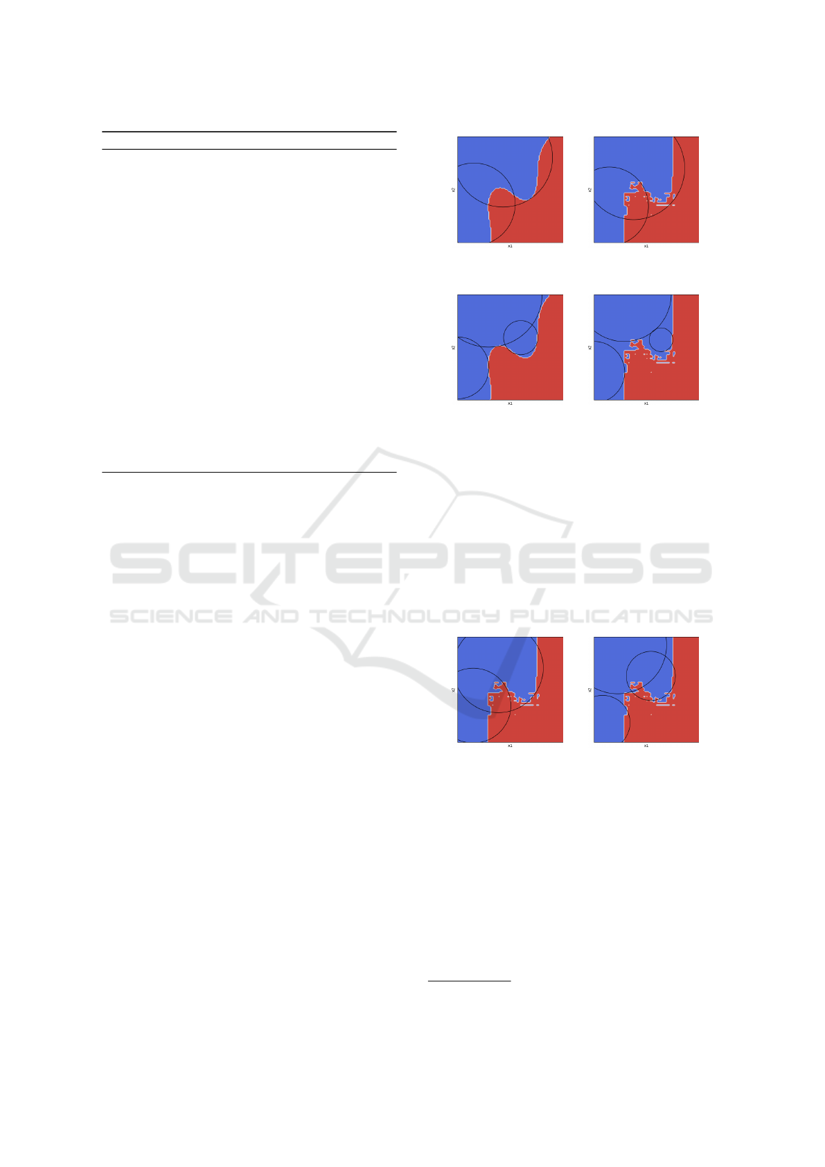
Figure 1 presents the HR hypersphere sets for each
classifier. Both HR hypersphere sets are constructed
with 5000 samples. The left of Figure 1 presents the
HR hypersphere set that fits SVC. In this condition,
the HR hypersphere set satisfies the ideal property (
Definition 1). However, the HR hypersphere set for
RF does not satisfy Definition 1 because it misses a
small blue region (right of Figure 1). Laugel(Laugel
et al., 2019) reports that an ensemble tree classifier
shows low robust boundary and it generates such a
region. We construct an HR hypersphere set by using
generated samples. Therefore, if samples do not exist
on such a region. Then it cannot capture the classi-
fier behavior An HR hypersphere set losses the ideal
property.
We construct an HP hypersphere set with 5000
samples as presented in Figure 2. The HP hyper-
sphere set for SVC satisfies Definition 3 (right of Fig-
ure 2), i.e. not every hypersphere includes red re-
gions. A hypersphere at the right of Figure 2 includes
a small incorrect region because no samples exists in
the red region.
Figure 1: High-recall hypersphere sets for black-box classi-
fiers: Left, SVC; Right, RF.
Figure 2: High-precision hypersphere sets for black-box
classifiers: Left, SVC; Right, RF.
In Figure 3, we present the HR and HP hyper-
sphere set that fits RF and constructed with a small
number of samples (100 samples). The HR hyper-
sphere set misses wider than the target region at the
right of Figure 1. Actually, the recall is decreased
from 1.00 to 0.98. Moreover, the HP hypersphere set
includes a wider incorrect regions than the right of
Figure 2. The precision is also decreased from 1.00
to 0.95. These issues arise because the number of
samples is insufficient. Samples cannot capture the
classifier behavior.
Figure 3: Hypersphere sets with a small number of samples:
Left, HR; Right, HP.
5.2 Evaluation of Reliability
We measure the reliability of the explanatory region
with the iris and wine dataset, which are opened in the
UCI machine learning repository
3
. Table 1 presents
details of the datasets. As black-box models, we
trained a SVC, multilayer perceptron (MLP), and RF
with default hyper-parameters of the scikit-learn li-
brary. We compared the proposed method to baseline
methods: BA-Tree (BA) (Breiman and Shang, 1996)
and DefragTrees (DT) (Hara and Hayashi, 2018). We
3
https://archive.ics.uci.edu/ml/index.php
ICAART 2022 - 14th International Conference on Agents and Artificial Intelligence
240

implemented BA-Tree and use Hara’s implementation
for DefragTrees. Regarding the parameters of the pro-
posed method, we generated 10000 samples to con-
struct hypersphere sets and used K = 10 and L = 10
for parameters.
We used metrics for reliability: recall (6) and pre-
cision (7). We evaluated coverage using the cov-
erage ratio: the true coverage over the estimated
coverage(8). As a validation set, we uniformly sam-
pled 50000 instances and produced ground truth with
an input model.
After we split a dataset to 80% training data and
20% test data. We computed metrics 10 times each
training/test split. The smallest size of the class is set
as the target class.
Table 1: Details of datasets: numbers of whole instances
and numbers of dimension.
datasets # d
Iris 150 4
Wine 178 13
Comparison with the recall is presented in Table 2.
An HR hypersphere set shows higher recall than any
other conditions. This fact indicates that an HR hy-
persphere set satisfies our required property: The ex-
planatory region covers the target region. An HP hy-
persphere set shows higher recall than BA-tree for the
Iris dataset with SVC and MLP. However it tends to
show low recall for the Wine dataset and RF. Espe-
cially, the BA-tree shows low recall under SVC and
MLP conditions. Therefore, BA is inappropriate for
non-rule classifier. DefragTrees is only applicable for
RF because it is model specific explanation method.
Table 2: Comparison of proposed method and baseline
methods with recall. The highest recall is shown in bold-
face.
HR HP BA DT
Iris SVC 0.998 0.761 0.610 –
MLP 0.997 0.783 0.726 –
RF 0.996 0.392 0.847 0.367
Wine SVC 0.911 0.196 0.088 –
MLP 0.976 0.197 0.087 –
RF 0.971 0.066 0.532 0.327
We present a comparison with precision in Ta-
ble 3. The HP hypersphere set shows the highest
precision expect for the Wine dataset and RF. There-
fore we can use an HP hypersphere set as a surro-
gate model. The HR hypersphere set tends to show
low precision. It indicates that an HR region includes
many incorrect regions. The BA-tree shows low pre-
cision under non-rule classifier conditions. The BA-
tree and DefragTrees show high precision for RF.
They use a rule model as an explanatory region and
perform high precision to explain ensemble tree mod-
els.
Table 3: Comparison of proposed method and baseline
methods with precision. The highest precision is shown in
boldface.
HR HP BA DT
Iris SVC 0.384 0.993 0.766 –
MLP 0.391 0.995 0.737 –
RF 0.434 0.990 0.927 0.948
Wine SVC 0.351 0.851 0.107 –
MLP 0.207 0.935 0.186 –
RF 0.187 0.770 0.659 0.935
Table 4 presents the comparison with the cover-
age ratio. The BA-tree shows the best coverage ratio
for Iris dataset. The HP hypersphere set shows the
best coverage for the Wine dataset with SVC and RF
conditions. However, it shows a bad coverage ratio
for RF. A greater than 1 coverage ratio of HR hyper-
sphere set means that its explanatory region includes
large incorrect regions.
Table 4: Comparison of proposed method and baseline
methods with coverage ratio. The best coverage ratio is
shown in boldface.
HR HP BA DT
Iris SVC 2.186 0.783 0.819 –
MLP 2.683 0.800 0.981 –
RF 2.436 0.479 0.941 0.388
Wine SVC 2.700 0.228 0.168 –
MLP 4.833 0.206 0.193 –
RF 5.215 0.076 0.859 0.359
6 CONCLUSIONS
We proposed a novel global explanation method using
hypersphere sets of two types. We defined the high-
recall and high-precision hypersphere set to reveal the
internal behavior of a black-box model. These hyper-
sphere sets are designed, respectively, to fit the super-
set and subset of the target region. To compute each
hypersphere set effectively, we introduce sample-
based notions and propose algorithms. Based on the
illustrative experiment, we demonstated that hyper-
sphere sets satisfy the necessary property. Moreover,
the proposed method exhibited higher reliability met-
rics than earlier reported global explanation methods.
As an application of our method, by clarifying the be-
havior of a model, it is possible to select an appropri-
ate model.
Post-hoc Global Explanation using Hypersphere Sets
241

Now, our method supports only numerical input.
Therefore to improve the range of application, it must
be extended to the mixed data input: numerical and
categorical data. Our method sometimes does not
work for the classifier that trained an imbalanced
dataset. Therefore, we have to improve the robust-
ness.
ACKNOWLEDGEMENTS
This work was partially supported by JSPS Kakenhi
20H04143 and 17K00002.
REFERENCES
Aivodji, U., Arai, H., Fortineau, O., Gambs, S., Hara, S.,
and Tapp, A. (2019). Fairwashing: the risk of ra-
tionalization. volume 97 of Proceedings of Machine
Learning Research, pages 161–170, Long Beach, Cal-
ifornia, USA. PMLR.
Angelino, E., Larus-Stone, N., Alabi, D., Seltzer, M., and
Rudin, C. (2017). Learning certifiably optimal rule
lists. In Proceedings of the 23rd ACM SIGKDD In-
ternational Conference on Knowledge Discovery and
Data Mining, pages 35–44. ACM.
Asano., K. and Chun., J. (2021). Post-hoc explanation us-
ing a mimic rule for numerical data. In Proceedings of
the 13th International Conference on Agents and Ar-
tificial Intelligence - Volume 2: ICAART,, pages 768–
774. INSTICC, SciTePress.
Asano, K., Chun, J., Koike, A., and Tokuyama, T. (2019).
Model-agnostic explanations for decisions using min-
imal patterns. In Artificial Neural Networks and Ma-
chine Learning – ICANN 2019: Theoretical Neural
Computation, pages 241–252, Cham. Springer Inter-
national Publishing.
Breiman, L. and Shang, N. (1996). Born again trees. Uni-
versity of California, Berkeley, Berkeley, CA, Techni-
cal Report.
Caruana, R., Lou, Y., Gehrke, J., Koch, P., Sturm, M., and
Elhadad, N. (2015). Intelligible models for healthcare:
Predicting pneumonia risk and hospital 30-day read-
mission. In Proceedings of the 21th ACM SIGKDD In-
ternational Conference on Knowledge Discovery and
Data Mining, pages 1721–1730. ACM.
Dash, S., Gunluk, O., and Wei, D. (2018). Boolean decision
rules via column generation. In Advances in Neural
Information Processing Systems, pages 4655–4665.
Deng, H. (2019). Interpreting tree ensembles with intrees.
International Journal of Data Science and Analytics,
7(4):277–287.
Dumitrescu, A. and Jiang, M. (2013). On the largest
empty axis-parallel box amidst n points. Algorith-
mica, 66(2):225–248.
Dyer, M. (1992). A class of convex programs with appli-
cations to computational geometry. In Proceedings of
the Eighth Annual Symposium on Computational Ge-
ometry, SCG ’92, page 9–15, New York, NY, USA.
Association for Computing Machinery.
Fischer, K., G
¨
artner, B., and Kutz, M. (2003). Fast smallest-
enclosing-ball computation in high dimensions. In
Proc. 11th European Symposium on Algorithms (ESA,
pages 630–641. SpringerVerlag.
Friedman, J. H. (2001). Greedy function approximation: a
gradient boosting machine. Annals of statistics, pages
1189–1232.
Guidotti, R., Monreale, A., Ruggieri, S., Pedreschi, D.,
Turini, F., and Giannotti, F. (2018a). Local rule-based
explanations of black box decision systems. arXiv
preprint arXiv:1805.10820.
Guidotti, R., Monreale, A., Ruggieri, S., Turini, F., Gian-
notti, F., and Pedreschi, D. (2018b). A survey of meth-
ods for explaining black box models. ACM Computing
Surveys (CSUR), 51(5):93.
Hara, S. and Hayashi, K. (2018). Making tree ensembles in-
terpretable: A bayesian model selection approach. In
Storkey, A. and Perez-Cruz, F., editors, Proceedings
of the Twenty-First International Conference on Ar-
tificial Intelligence and Statistics, volume 84 of Pro-
ceedings of Machine Learning Research, pages 77–
85. PMLR.
Lakkaraju, H., Aguiar, E., Shan, C., Miller, D., Bhanpuri,
N., Ghani, R., and Addison, K. L. (2015). A ma-
chine learning framework to identify students at risk
of adverse academic outcomes. In Proceedings of
the 21th ACM SIGKDD international conference on
knowledge discovery and data mining, pages 1909–
1918. ACM.
Lakkaraju, H., Bach, S. H., and Leskovec, J. (2016). Inter-
pretable decision sets: A joint framework for descrip-
tion and prediction. In Proceedings of the 22nd ACM
SIGKDD international conference on knowledge dis-
covery and data mining, pages 1675–1684. ACM.
Laugel, T., Lesot, M.-J., Marsala, C., Renard, X., and De-
tyniecki, M. (2019). The dangers of post-hoc inter-
pretability: Unjustified counterfactual explanations.
In Proceedings of the Twenty-Eighth International
Joint Conference on Artificial Intelligence, IJCAI-19,
pages 2801–2807. International Joint Conferences on
Artificial Intelligence Organization.
Lundberg, S. M., Erion, G., Chen, H., DeGrave, A., Prutkin,
J. M., Nair, B., Katz, R., Himmelfarb, J., Bansal, N.,
and Lee, S.-I. (2020). From local explanations to
global understanding with explainable ai for trees. Na-
ture machine intelligence, 2(1):56–67.
Lundberg, S. M. and Lee, S.-I. (2017). A unified approach
to interpreting model predictions. In Advances in neu-
ral information processing systems, pages 4765–4774.
Pedreschi, D., Giannotti, F., Guidotti, R., Monreale, A.,
Ruggieri, S., and Turini, F. (2019). Meaningful expla-
nations of black box ai decision systems. In Proceed-
ings of the AAAI conference on artificial intelligence,
volume 33, pages 9780–9784.
Ribeiro, M. T., Singh, S., and Guestrin, C. (2018). An-
chors: High-precision model-agnostic explanations.
In AAAI, pages 1527–1535.
ICAART 2022 - 14th International Conference on Agents and Artificial Intelligence
242

Roscher, R., Bohn, B., Duarte, M. F., and Garcke, J. (2020).
Explainable machine learning for scientific insights
and discoveries. Ieee Access, 8:42200–42216.
Rudin, C. (2019). Stop explaining black box machine learn-
ing models for high stakes decisions and use inter-
pretable models instead. Nature Machine Intelligence,
1(5):206–215.
Rudin, C. and Shaposhnik, Y. (2019). Globally-consistent
rule-based summary-explanations for machine learn-
ing models: Application to credit-risk evaluation.
SSRN Electronic Journal.
Wang, F. and Rudin, C. (2015). Falling rule lists. In Artifi-
cial Intelligence and Statistics, pages 1013–1022.
Wang, T. (2018). Multi-value rule sets for interpretable
classification with feature-efficient representations. In
Bengio, S., Wallach, H., Larochelle, H., Grauman, K.,
Cesa-Bianchi, N., and Garnett, R., editors, Advances
in Neural Information Processing Systems 31, pages
10835–10845. Curran Associates, Inc.
Welzl, E. (1991). Smallest enclosing disks (balls and ellip-
soids). In Maurer, H., editor, New Results and New
Trends in Computer Science, pages 359–370, Berlin,
Heidelberg. Springer Berlin Heidelberg.
Zhao, Q. and Hastie, T. (2021). Causal interpretations of
black-box models. Journal of Business & Economic
Statistics, 39(1):272–281.
Post-hoc Global Explanation using Hypersphere Sets
243