Optimization of Sensor Placement for Birds Acoustic Detection in

Complex Fields

Damien Goetschi

, Val

ere Martin

, Richard Baltensperger

, Marc Vonlanthen

Donatien Burin des Roziers

and Francesco Carrino

1,3 a

University of Applied Sciences and Arts Western Switzerland, CH-1700 Fribourg, Switzerland

Nos Oiseaux, CH-2300 La Chaux-de-Fonds, Switzerland

University of Applied Sciences and Arts Western Switzerland,CH-1950 Sion, Switzerland

Keywords:

Modeling of Sound Propagation, Sensor Placement Optimisation, Particle Swarm Optimization, Genetic

Algorithms, Bird Conservation.

Abstract:

Birds nest in multifunctional semi-natural environments. Intensiﬁcation of agriculture and forestry prevents

their successful breeding, threatening globally their survival. Early bird detection allows for targeted conser-

vation actions, such as local (temporary) habitat protection. The conservationist thus looks for at detecting

priority bird species as soon as a territory is occupied, for instance using acoustic surveillance network. We

present a comprehensive method to optimize acoustic coverage with a minimum number of sensors in the

network. Our method includes a sound propagation model and algorithms for optimized sensor placement.

Relevant parameters (e.g., topography, soil type, height of vegetation, weather, etc.) for the sound propagation

model are automatically extracted from an area of interest. We implemented and compared Particle Swarm

Optimization and Genetic Algorithms-based approaches to solve the optimisation problem.

1 INTRODUCTION

Birds breeding in Switzerland occupy forest and

farming environments exploited as well for natural

resources. The intensive operations on such lands

strongly jeopardize their breeding success. Threat-

ened species are for instance the Corncrake (Crex

crex) or the Eurasian Pygmy-owl (Glaucidium passer-

inum). Early detection, accurate localization, detailed

behavioral information and proper policy applications

altogether allow to enforce permanent or temporary

habitat protection and disturbance avoidance for suc-

cessful nesting. This paper topic deals with early

detection using acoustic network made up of many

acoustic sensors in order to survey an area of interest.

Two main practical questions arise: how many and

where should the sensors be located ? Which portion

of the area is actually covered (coverage) ?

Given an area of interest, the problem of exhaus-

tive bird detection through acoustic sensors is partic-

ularly challenging since it requires to precisely model

sound propagation in complex and heterogeneous nat-

https://orcid.org/0000-0003-0152-2161

ural environments. Sound propagation depends on

factors such as weather, elevation, type of vegetation,

etc. Without the knowledge of the sensors’ real de-

tection range (as modiﬁed by the above-mentioned

factors), either birds are unknowingly missed or the

number of acoustic devices to completely cover the

area will be excessively high. The main objective of

this paper is to present a tool for the optimized conﬁg-

uration of large autonomous acoustic monitoring net-

works for bird detection.

We propose to model sound propagation ac-

cording to the ISO 9613-2 standard (ISO 9613-

2:1996(F), 1996) and to computationally search for

a near-optimal sensor location given a number of

available sensors. For this purpose, we imple-

mented particle swarm optimization (PSO) algorithm

(Bonyadi and Michalewicz, 2017) and genetic algo-

rithms (GAs) (Whitley, 1994) (detailed information

about our methodology is provided in Section 3).

To validate our approach, we developed a tool

that, given the geographical coordinates of an area

of interest, the number of available sensors and their

speciﬁcations (such as the detection range), automat-

ically collects all the relevant ﬁeld information and

550

Goetschi, D., Martin, V., Baltensperger, R., Vonlanthen, M., Roziers, D. and Carrino, F.

Optimization of Sensor Placement for Birds Acoustic Detection in Complex Fields.

DOI: 10.5220/0010819000003122

In Proceedings of the 11th International Conference on Pattern Recognition Applications and Methods (ICPRAM 2022), pages 550-559

ISBN: 978-989-758-549-4; ISSN: 2184-4313

computes a near-optimal solution for the network

conﬁguration. For practical use, the tool allows as

well manual adaptation of the proposed solution to

consider possible unforeseen practical ﬁeld problems

(e.g., a sensor’s computed location is inaccessible or

on a private land).

This paper is structured as follow: Section 2

presents the state of the art concerning the mod-

eling of sound propagation, the theories supporting

near-optimal sensor placement, and computational

methods to solve such a problem; Section 3 details

the sound propagation model we adopted (i.e., ISO

9613-2), the sensor placement algorithm, the archi-

tecture of our system and how we adapted PSO and

GAs approaches for our coverage problem; Section

4 presents and discusses the results. Finally, in Sec-

tion 5, we present the limitations and outlooks of our

work.

2 STATE OF THE ART

To the best of our knowledge, no systematic and rig-

orous method for deploying acoustic monitoring net-

works for ornithology has been yet developed. Such

a method implies two main tasks: 1) describing how

the sound travel in a heterogeneous landscape and 2)

how to use this information to place the sensors in

the ﬁeld in order to minimize the probability of unde-

tected sound.

In this section, we brieﬂy present recent works

on sound propagation models, probabilistic theory of

sensor placement and acoustic coverage optimisation

methods.

2.1 Sound Propagation

Modeling the propagation of sound is a complex prob-

lem that depends on many parameters such as the fre-

quency and sound pressure at the source, the meteo-

rological conditions, the nature of the ground and the

obstacles encountered by the sound or the relief. Tak-

ing into account all these parameters implies in return

to account for physical phenomena such as reﬂection

and diffraction of sound waves, wind speed proﬁles

and turbulence, geometric dispersion or absorption of

sound energy by atmospheric molecules.

Analytical and numerical approaches have been

developed and applied in order to tackle the prob-

lem of sound propagation. Selection of one approach

mainly depends on the complexity of the particular

situation as well as on the computer resources avail-

able.

Analytical methods are often based on geometri-

cal acoustics and are therefore relevant for simple sit-

uations involving an homogeneous and isotropic at-

mosphere, an homogeneous ground and a zero or con-

stant vertical gradient of sound speed (Attenborough

et al., 1980; de Hoop et al., 2005). Geometrical acous-

tics relies on the ray tracing theory that assumes sound

to be a large number of very narrow beams propagat-

ing in a straight light unless it encounters an obstacle

or a change in the medium of propagation. Propaga-

tion above a mixed ground is more complex and has

also been studied using Green formulation (Chandler-

Wilde and Hothersall, 1985).

In the last few years, propagation of sound in com-

plex ﬁelds including heterogeneous grounds and me-

teorological events has been widely studied. The de-

veloped numerical methods have also been compared

with the analytical approaches and with ﬁeld mea-

surements.

The Fast Field Program (FFP) is a computational

technique involving the Hankel transformation of the

Helmholtz equation in circular cylindrical coordinates

and the integration of the resulting ordinary differen-

tial equation by analogy with electrical transmission

lines (Raspet et al., 1985).

Boundary Elements Methods (BEM) approxi-

mates the solutions of partial differential equation im-

plied in the sound propagation by looking at their so-

lutions at the boundaries of the discretized elements

of the space. The accuracy of these methods has been

well validated against other numerical models (Lam

and Monazzam, 2006).

The Transmission Line Matrix method (TLM)

(Guillaume et al., 2014) or the Meteo-BEM (Premat

and Gabillet, 2000) provide other examples of numer-

ical methods that have been applied to sound propa-

gation.

Nevertheless, these numerical approaches are time

and computer resources consuming. Moreover, their

implementation becomes very fastidious when con-

sidering complex environments, mixed inﬂuence of

terrain topography and time-dependent atmospheric

conditions. An alternative is to consider in an incre-

mental way the different contributions (geometrical

dispersion, atmospheric absorption, ground effects,

etc.) to sound attenuation and to subtract them form

the sound pressure at the source. This is the method

supported by the International Organisation for Stan-

dardization (ISO) which is commonly used in engi-

neering (ISO 9613-2:1996(F), 1996).

Optimization of Sensor Placement for Birds Acoustic Detection in Complex Fields

551

2.2 Theory of Sensor Placement

A key question in the ﬁeld of acoustic network de-

tection is where one should place the sensors in order

to maximize the chance of detecting the event of in-

terest, in our case a bird song. There are different

approaches to tackle this question.

One possible approach is to assume that sensors

have a ﬁxed sensing radius and to solve the task as an

instance of the art-gallery problem (Gonz

alez-Banos,

2001). The problem with this approach is that the ge-

ometrical assumption is too strong and cannot suc-

cessfully be applied in very complex ﬁeld where the

sensing range is not constant and depends on local en-

vironmental conditions. An alternative approach from

spatial statistics (Caselton and Zidek, 1984) assumes

weaker geometrical assumptions. It relies on a pilot

deployment or expert knowledge to train a gaussian

process model that allows for localization predictions

made over the sensed ﬁeld. The model can then be

used to predict the effect of placing sensors at partic-

ular locations, and thus optimize their positions. For

a given gaussian process model, different criteria can

be proposed to ﬁnd the optimal sensor placement. A

criteria that is often used is entropy: highest entropy

corresponds to regions where the sensors are most un-

certain about each other’s measurements. The typical

sensor placement technique is to greedily add sensors

where the entropy is maximal (Cressie and Moores,

2021). However, in our case, the entropy criteria does

not seem to be relevant since the set of sensors is

then characterized by sensor locations that are as far

as possible from each others. This results in sensors

distributed at the border of the region of interest (Ra-

makrishnan et al., 2005).

In (Krause et al., 2008), the authors present a

greedy-heuristic method based on maximizing the

mutual information between the chosen location and

those which are not selected yet. This approach has

then successfully been applied for determining near-

optimal placement of acoustic devices for monitor-

ing wildlife resources and for localization of sound

sources (Pi

na-Covarrubias et al., 2019).

2.3 Particle Swarm Optimization and

Genetic Algorithms for

Mathematical Optimization in

Sensor Networks

Mathematical optimization consists in the selection

of the best element in the space of possible solutions

(Yang, 2008). The elements are ranked via an objec-

tive function (also called ﬁtness function, loss func-

tion or cost function, depending on the context and

goals). The space of possible solution is typically lim-

ited by some constraints. Many methods exist to ﬁnd

optimal or pseudo-optimal solutions. In this work, we

use and compare two approaches: particle swarm op-

timization (PSO) and genetic algorithms (GAs).

PSO (Kennedy and Eberhart, 1995) is a compu-

tational method used in many domains (Bonyadi and

Michalewicz, 2017) that aims to solve iteratively an

optimization problem by “moving” a population of

possible solutions, called “particles”, in the space of

possible solutions. Simple mathematical formulas

manage each particle’s position and velocity. Each

particle is “attracted” in a direction that depends on

the position of its personal (or local) best and the

position of the current global best discovered by the

swarm (any particle). This is expected to move the

swarm towards the best solutions. A good combina-

tion of hyper-parameters such as number of iterations,

number of particles, inertia weight, acceleration coef-

ﬁcients, etc. is very important to cover the full space

of possible solutions and to converge while avoiding

local optima.

GAs (Whitley, 1994) is a family of computational

methods that aim to solve iteratively an optimization

problem by following a process inspired by Charles

Darwin’s theory of natural selection. The main idea

is to select from the population (i.e., a large group

of possible solutions) the best individuals and mixing

their “chromosomes” (i.e., their features) in a smart

way to generate an improved second generation. Gen-

eration by generation, the algorithm should converge

to the global optimum. A good combination of hyper-

parameters such as number of generations, the popu-

lation size, methods used for the selection, modiﬁca-

tion and transmission of the chromosomes (crossover,

recombination and mutation) may help the algorithm

to converge while avoiding local optima.

In an abstract way, it is possible to see PSO as

a particular case of GAs, in which the swarm size

corresponds to the population size and the logic used

to compute the particles displacement corresponds to

particular crossover and mutation strategies.

Since more than 20 years, PSO and GAs have

been proposed to solve node placement problems in

Wireless Sensor Networks (WSN). In (Younis and

Akkaya, 2008) (2008), Younis and Akkaya presented

a survey about strategies and techniques for node

placement in WSN. Their survey is very broad, cov-

ering the problem of maximal coverage of the moni-

tored area (with the lower number of sensors). How-

ever, they clearly present how the choice of the de-

ployment scheme depends on the application, the ty-

pology of sensors, and the environment. They sug-

ICPRAM 2022 - 11th International Conference on Pattern Recognition Applications and Methods

552

gest to prefer deterministic approaches when sen-

sors are expensive or when their performances are di-

rectly impacted by their position as in our case. Con-

cerning PSO, (Kulkarni and Venayagamoorthy, 2010)

presents a survey about the use of PSO for the place-

ment of stationary and mobile nodes, along with other

PSO based solutions for WSN problems such as data

aggregation, node localization and energy-aware clus-

tering. They showed that PSO is a suitable approach

to solve optimization problems in WSNs due to “its

simplicity, high quality of solution, fast convergence,

and insigniﬁcant computational burden”. However,

they also raise awareness about its limitations for

high-speed real-time applications given the iterative

nature of PSO.

GAs have been successfully applied in many con-

texts (machine learning, scheduling, placement) and

domains (engineering, biology, and medicine) (Ay-

bars, 2008). In 2020, ZainEldin et al. (ZainEldin

et al., 2020) presented a comparison between different

state-of-the-art GA-based techniques used for place-

ment of WSN. In their analysis, they classiﬁed algo-

rithms according to three aspects: coverage, connec-

tivity and minimum number of nodes. Most of the

approaches proposed successfully achieved full cov-

erage while minimizing cost (e.g., the number of de-

ployed sensors). However, they did not all consider

all the three aspects and most of them developed ﬁt-

ness functions and crossover approaches speciﬁc for

their problem. In our work, we focus on the cover-

age problem while taking into account outdoor envi-

ronment factors such as elevation, vegetation height

and density, average weather conditions, etc. In this

same direction, (Pal et al., 2021) recently faced sim-

ilar challenges for the deployment of sensor nodes

communicating under IEEE 802.15.4 wireless stan-

dard. They successfully build a reliable WSN for crop

monitoring, but their focus was more to keep connec-

tivity between sensors than on coverage aspects.

3 METHODOLOGY

3.1 Sound Propagation Model

Concerning the sound propagation model and for the

sensor placement algorithm (see Section 3.2), we

adopt the methodology from (Pi

na-Covarrubias et al.,

2019). Since these different elements of the model

are separately implemented in our algorithm, they can

easily be changed or improved in further develop-

ments.

We use fundamental equations according to ISO

9613-2 (ISO 9613-2:1996(F), 1996). We need to cal-

culate the sound pressure L

in decibels at the position

of the sensor as a function of the sound pressure L

at the emitter, possible corrections D due to the direc-

tivity of the source and some attenuation factors A

the sound between the source and the sensor:

= L

+ D −

∑

(1)

Since we consider the sound sources as emitting

with no preferred direction, D = 0 dB. The attenua-

tion factors A

may depend on the frequency of the

sound. The ﬁrst of these factors A

comes from the

geometrical spreading of the sound into space. It de-

pends on the distance d between the source and the

sensor and of some reference distance d

set to 1 m:

= 20 log





+ 11 (2)

The second factor A

is a consequence of atmo-

spheric attenuation which converts sound energy into

heat. It depends strongly on the distance d, the sound

frequency and some meteorological parameters like

humidity and air temperature. Therefore

= αd (3)

where α is a coefﬁcient that takes into account these

dependencies. The third factor A

is the ground effect

because of the reﬂections of the sound on the ground.

It can be written as

= A

+ A

(4)

where A

, A

and A

are speciﬁc contributions to

the ground attenuation at the source, at the receiver

and in an intermediate position, respectively.

The fourth one, A

, is the attenuation occurring

in the presence of vegetation. In accordance with the

ISO 9613-2 standard, it depends strongly on the fre-

quency and on the distance d

travelled by the sound

in the vegetation. Attenuation from vegetation con-

tributes in a limited way to the overall attenuation.

Typical values are of the order 1-2 dB. Some cor-

rections C

weather

from the meteorological conditions

are also taken into account. But as it is emphasized

in (ISO9613 − 2 : 1996(F), 1996), experience shows

that those corrections are, in practice, limited to the

range from 0 to about 5 dB and values above 2 dB are

exceptional.

Figure 1 shows the effects of each attenuation on

a given sound as the distance increases. A

due to

geometrical spreading of sound is by far the most im-

portant contribution to the sound attenuation.

Optimization of Sensor Placement for Birds Acoustic Detection in Complex Fields

553

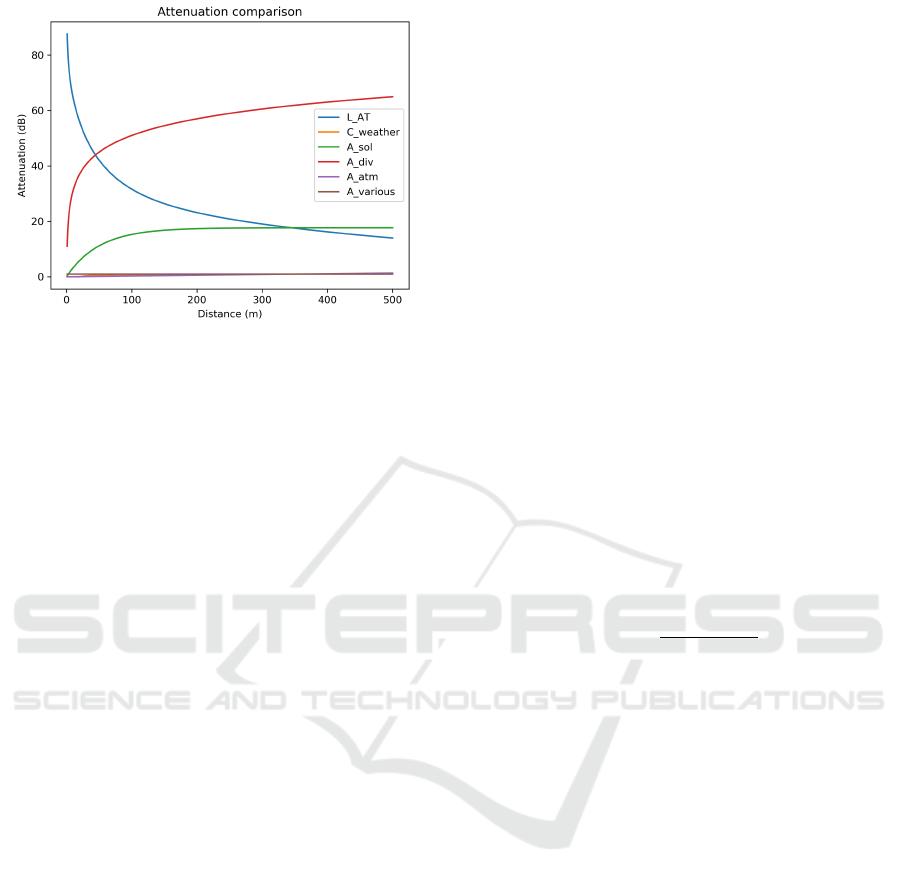
Figure 1: Comparison of the different attenuation contri-

butions to sound intensity. Here, L

is the overall sound

attenuation (L

in equation (1)), A

sol

= A

is the ground at-

tenuation, A

div

= A

the geometrical spreading, A

atm

= A

the atmospheric absorption and A

various

the other less sig-

niﬁcant attenuation factors.

3.2 Sensor Placement Algorithm

We present here the main results of the sensor place-

ment algorithm developed in (Pi

na-Covarrubias et al.,

2019) and that we adapted in our system. A given

region is considered with a set G of possible sound

sources and a set D of possible sensor placements.

The goal of this approach is to minimize the proba-

bility of not detecting a sound emitted somewhere in

G. The probability of detecting a sound that occurs at

any location i ∈ G when a single sensor is deployed

at location j ∈ D is given by

∑

i∈G

i, j

(5)

where P

i, j

is a function depending on the sound

pressure level detected at j ∈ D of a sound emitted

at i ∈ G. The sound pressure is computed with the

method described in Section 3.1. If n devices are de-

ployed on a set of possible locations N , the probabil-

ity of at least one sensor detecting a sound occuring

at any location in G is

= 1 −

∑

i∈G

∏

j∈N

1 − P

i, j

. (6)

Equation (6) assumes independent sound detec-

tion by each sensor.

The algorithm then proceeds by iterative greedy

placement of the n sensors in order to maximize the

probability P

in Equation (6). In case n = 1, the

problem is easily solved by choosing the single loca-

tion in D that maximizes the probability, but for n ≥ 1

the problem is more complex. It becomes then combi-

natorial in the sense that the algorithm has to evaluate

the probability for n locations over all the set of pos-

sible locations in D. The iteration allocates the ﬁrst

of the n sensors for which the probability of not miss-

ing a sound is the highest (or, in other terms, it places

the sensor that minimizes the probability of missing

a rare sound). Then, at each iteration, it ﬁnds the op-

timal location for the next sensor given the position

of the previously placed ones. The result from this

greedy approach has been proved to be close to the

optimal placement (Krause et al., 2008).

Once the optimal sensor placement has been de-

termined, the next step consists in the sound localiza-

tion. Considering a subset of the deployed sensor at

locations N

∈ N . If one or more of these sensors de-

tect the sound, while the others at locations N \ N

fail to detect the sound, the likelihood that these ob-

servations were caused by a sound emitted at location

i ∈ G is

∏

j∈N

i, j

∏

j∈N \N

1 − P

i, j

(7)

Given that and using Bayes’ theorem, the poste-

rior probability P

that the sound was emitted at lo-

cation i is

∑

i∈G

(8)

If more that one sensors detects the sounds and

the time of each detection is available, then it is pos-

sible to extend the analysis and to reﬁne the model

proposed using Equation (8). However, this has not

been implemented yet in our algorithm and the de-

tails of the enlarged procedure are explained in (Pi

na-

Covarrubias et al., 2019).

3.3 System Description

In order to ﬁnd the best sensors locations, a user has to

provide to the system information such as the region

of interest, the sensors’ speciﬁcations and the charac-

teristics of the targeted species: where the bird sings

(on the ground, while ﬂying, in the bushes, etc.), the

sound frequency (Hz) and the average sound pressure

level at the source (dB).

As explained in Section 3.1, the sound propaga-

tion model requires information about the topography,

vegetation height/type (ﬁelds, forest, bushes, etc.) and

the meteorological conditions on site. This informa-

tion is used to deﬁne the probability matrix for all pos-

sible sound sources G (see Section 3.4). Once deﬁned

the perimeter of the region of interest (in terms of

ICPRAM 2022 - 11th International Conference on Pattern Recognition Applications and Methods

554

latitude-longitude coordinates), the system automati-

cally gathers all the information required for the com-

putation.

The ﬁrst source of information is Swisstopo (Fed-

eral Ofﬁce of Topography, 2021). Available data on

topography and vegetation have a resolution of half

a meter. The second source is IDAweb from Me-

teoSwiss (Swiss Federal Ofﬁce of Meteorology and

Climatology) providing data collected by ground sta-

tions. Concerning the weather data, since the sen-

sors have to remain on site for long time intervals,

we use monthly-averaged temperature, humidity and

pressure.

Given this information, our tool provides the esti-

mated best location in which to place the sensors and

the expected coverage. Finally, even if our tool is not

yet intended for the use of general public, we devel-

oped a minimal user interface that allows manually

changing the position of each sensors, recomputing

“on-the-ﬂy” the expected coverage. This allows con-

sidering possible difﬁculties encountered in the ﬁeld

such as unreachable areas, unexpected noisy environ-

ments, etc.

3.4 Optimisation Algorithms: Concept

and Implementation

The main idea of our work is to combine the al-

gorithm proposed in Section 3.2 (Pi

na-Covarrubias

et al., 2019) with the computational mathematical op-

timization methods presented in Section 2.3 while us-

ing the ISO 9613-2 sound propagation model (Section

3.1).

In the ﬁrst step, the information contained in the

map (elevation, vegetation height, weather, etc.) are

combined with information coming from the bird pro-

ﬁle. This operation provides a probability matrix that

covers all the area and it models the probability dis-

tribution of the presence of a given species of birds

(it corresponds to P

in Equations (5) and (6)). The

speciﬁcations of the sensors (e.g., sensibility, height

from ground, etc.) and the ISO 9613-2 sound propa-

gation model are then used to compute P

in Equa-

tion (6). As mentioned above, given a particular sen-

sor placement, P

represents the probability of miss-

ing a rare sound (in our case, a bird singing). This

function represents the core of the ﬁtness function that

our algorithms will try to minimize.

As introduced above, in this work we used and

compared PSO and GAs.

Concerning PSO, we used the standard formu-

lation with constraints support as implemented in

the pyswarm library (tisimst, 2015). We determined

hyper-parameters such as swarm size, max iterations,

ω, φ

, and φ

in a validation set composed of test

maps close but not overlapping the regions of interest.

ω, φ

and φ

represent “exploration versus exploita-

tion” parameters. They indicate the velocity of each

particle and the weight given by each particle to the

particle’s best known-position (current personal best)

and the swarm best-known position (current global

best) in order to compute their position at the next

iteration. In our problem, each particle represents the

possible placement of a sensors in the map. When

the algorithm converges or after the maximum num-

ber of allowed iterations (indicated by the parame-

ter max iterations), we select the swarm’s best-known

position as the position in which to place the sensor.

With this approach, sensors can be placed one after

the other to reach the desired number of sensors or,

possibly, until the ﬁtness function does not overcome

a given threshold. As a variant, we implemented a

“non-greedy” version of the same algorithm in which

we could place the n sensors at the same time. In the

greedy algorithm, once a sensor is placed, it cannot be

moved anymore, limiting the possibility to converge

to the actual global maximum that considers all the

sensors at once. In the second, non-greedy variant,

each particle represents the positioning of n sensors

at once. Our hypothesis is that it should not suffer

of the same limitation and converge to a better global

optimization. However, the problem that has to be

solved in each iteration becomes increasingly com-

plex (depending on the number of sensors to place at

once), therefore we expect to get better performance

but only after longer execution time.

Concerning the GAs, we needed an additional step

to formulate the problem in a way that could be solved

by an evolutionary approach. In particular, we needed

to deﬁne what represents an individual (or a chromo-

some) and, subsequently, the mathematical way to im-

plement crossover, recombination and mutation.

We considered an individual as a sensor posi-

tioned on the map. The individual’s chromosome rep-

resents its coordinates x, y. The population repre-

sents a set of individuals (i.e., a set of possible sen-

sor’s placement on the map). From the initial popu-

lation, we need to select the best elements that will

go through the crossover phase. To do this, we used

the approach known as “tournament selection”. This

method consists of randomly selecting a few individ-

uals and, among them, selecting those with a bet-

ter score in terms of the chosen ﬁtness function (the

“winners” of the tournament). This process is re-

peated many times and the winners of each tourna-

ment are designated for crossover. During crossover,

two individuals are selected at a time and they will

generate two new individuals of the next generation.

Optimization of Sensor Placement for Birds Acoustic Detection in Complex Fields

555

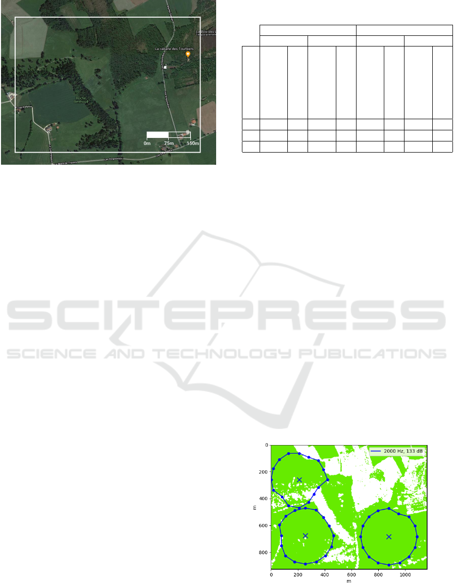
Figure 2: Region used for the test. As reference, the posi-

tion of orange point visible in the ﬁgure above is at coordi-

nates (46.972281 N, 6.704513 E).

The crossover function we implemented consists in a

weighted average among the chromosomes (i.e., the

coordinates) of the two parents, in which the weights

are random values between 0 and 1. In other terms,

this means that the offspring is placed in a random

position along a vector joining the two parents. Fi-

nally, the offspring has a given probability to present

mutations. Mutations are typically used to avoid local

maxima. In our case, a mutation consists in a ran-

dom offset along x and/or y that we added to the off-

spring. Once the mutation step is completed, we have

a new generation of individuals and the whole process

is repeated for a ﬁxed number of generations. From

this perspective, it is easy to see the correspondence

between swarm size in PSO and population size in

GAs, number of iterations (PSO) and number of gen-

erations (GAs). We kept these parameters consistent

between the two approaches in order to get more com-

parable results.

4 RESULTS AND DISCUSSION

To test and compare PSO’s and GAs’ “greedy” and

“non-greedy” versions, we used an area of one square

kilometer (Figure 2). We tested with up to 20 sen-

sors to evaluate the evolution of performance in terms

of coverage and time when increasing the number of

sensors. As the algorithms use random initialization

and may converge to different local optima after each

execution, we repeated each test 10 times and we av-

eraged the scores.

Table 1 presents a comparison between greedy and

non-greedy approaches using our PSO and GAs se-

tups. The test was carried out on the region speciﬁed

on Figure 2. The scores in the table represent:

Table 1: Comparison of versions and algorithms. Here, the

coverage represents the probability to detect a sound.

Greedy Non-greedy

PSO Genetic PSO Genetic

Number of sensors

coverage

time (min)

coverage

time (min)

coverage

time (min)

coverage

time (min)

3 51% 33 50% 20 49% 45 46% 29

4 61% 39 59% 25 60% 58 53% 33

5 69% 45 68% 29 65% 70 64% 42

• The overall coverage. It represents the probability

to detect a sound. It is computed as the ratio be-

tween the surface covered by the sensors and the

total surface, while considering the probability of

a sound to be emitted in each given point.

• The execution time. As a reference, all computa-

tions were done on the same machine and with-

out other applications running: CPU: 3.60 GHz,

RAM: 32 GB, OS: Windows 10.

Figure 3 presents the optimal sensors placement

for three sensors found by greedy genetic algorithm

on the region of Figure 2. As expected, the constant

133 dB sound pressure level (blue line) is closer to a

circular geometry around the sensor in case of an ho-

mogeneous ﬂoor and topography (e.g., the third sen-

sor at the bottom right on Figure 3).

Moreover, in this precise case, the target bird

species is known not to live in forest environments.

Therefore, the forest area present in the region was

excluded of the simulation. As shown in Table 1, the

coverage for three sensors using the greedy genetic al-

gorithm is about 50% determined in a time of 20 min-

utes. The coverage with the greedy PSO algorithm

Figure 3: Optimal placement of three sensors. The differ-

ent background colors are related to the vegetation height.

The blue line represents the same sound pressure level. Non

circularity around the sensor is due to unequal sound prop-

agation over different ﬂoors.

ICPRAM 2022 - 11th International Conference on Pattern Recognition Applications and Methods

556

is slightly better with 51%, but the time is then 33

minutes. Taken coverage and time consumption into

account lead to the conclusion of a better efﬁciency

for the greedy genetic approach.

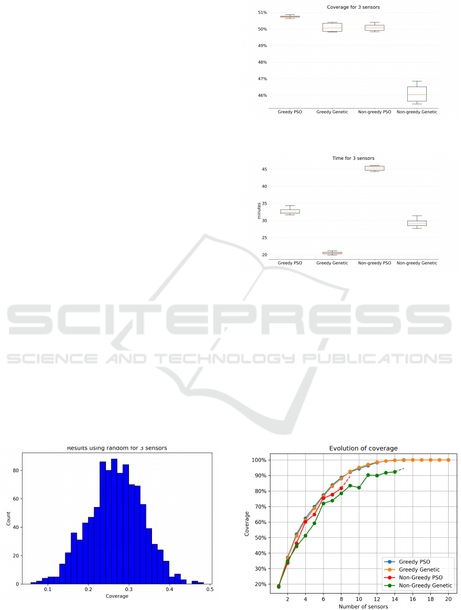
It is also relevant to compare our results with a

random placement of the sensors in terms of cover-

age. Results can be seen on Figure 4. Random sensor

placement was ran 1000 times and gave a coverage

mean value of 26% and a best value of 48% occur-

ring only once. The coverage obtained by our tests

presented in Table 1 are all above the random cover-

age distribution. This result gives an indication on the

validity of our different approaches.

As we see from Figures 5 and 6, in general, the

non-greedy methods that we proposed take more time

and give poorer results compared to greedy methods.

In the region of interest, with three sensors deployed,

PSO and GAs with greedy method provide a mean

coverage above 50%. GAs seems to have an cover-

age of 1 or 2% below but they take 40% less time.

Therefore, the choice of the most suitable algorithm

depends on the time available and how good the re-

sult has to be. It is also worth mentioning the nar-

rower coverage distribution of the greedy PSO al-

gorithm in comparison with the others ones. This

means that through the different runs, the PSO algo-

rithm tended to converge to the same, good solution

with low variance. However, the difference with the

other approaches remains small, of the order of a few

percent. As already emphasized, all approaches are

largely better than random placement (Figure 4).

Finally, Figures 7 and 8 show the coverage

and time-dependency of the different methods when

adding new sensors. Each color line corresponds to

the speciﬁed algorithm. On Figure 7, the different

points on each color line respectively indicate from

left to right the coverage for 1 and more sensors. For

Figure 4: Coverage distribution of random placement. Ran-

dom placements never reach the coverage of our algorithms

presented in Table 1.

Figure 5: Box plot of the coverage for each method. Mean

values can be found in Table 1.

Figure 6: Box plot of the time for each method. Mean val-

ues can be found in Table 1.

small numbers of sensors, we see that the coverage

still increases signiﬁcantly. However, as expected,

from a certain number of sensors, the region’s cov-

erage is reaching its saturation point (close to 100%

in our case study) and adding further sensors do not

bring any signiﬁcant improvement while leading to

an ever increasing computing time as it can easily

be seen from Figure 8. Indeed, with the same pre-

sentation, Figure 8 exhibits an ”almost linear” time-

dependency relative to the number of sensors. Imple-

menting a general method allowing us to ﬁnd an opti-

Figure 7: Evolution of coverage for all methods related to

number of sensors.

Optimization of Sensor Placement for Birds Acoustic Detection in Complex Fields

557

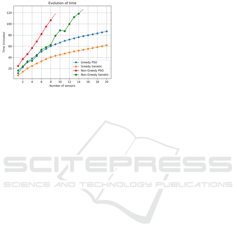
Figure 8: Evolution of time for all methods related to num-

ber of sensors.

mum between the number of sensors, the computing

time and the coverage will be the subject of further

developments. It is furthermore always possible to

add one or more sensors in our simulations. But for

the practical use of bird conservation for which our

system is intended, the number of detectors available

is often given by the means of ornithologists and re-

mains limited to a few units.

5 CONCLUSIONS

Acoustic recording is a widely used method for bird

conservation because of its low-cost. To scale-up

this method towards large networks, one central issue

is how to conﬁgure the network for the best cover-

age and the lowest number of recording devices. We

have developed a practical conﬁguration method suit-

able for various realistic situations. This method pro-

vides a high level of conﬁdence on the true acous-

tic coverage, which is particularly relevant in order to

demonstrate bird absence or scarcity. As such, this

tool entails a strong conﬁdence level with respect to

bird occurrence and thus strongly support bird pop-

ulation monitoring and conservation. The proposed

solution will be proof tested in the ﬁeld, using addi-

tional control devices within a test network and arti-

ﬁcial sounds. The test will also allow to estimate the

impact on detection caused by by wind, rain or an-

thropogenic noise.

Being mostly conceived for urban environments,

the ISO 9613-2 sound propagation model allows con-

sidering additional aspects such as reﬂections and bar-

riers. For our application in mostly natural land-

scapes, the current solution does not integrate these

aspects. However, it could be interesting to consider

them to increase the accuracy of our model in hybrid

landscapes where nature and buildings are mixed.

The modularity of the proposed architecture eas-

ily allows testing the same approaches while swap-

ping one of its components. New sound propagation

models can replace or extend the ISO 9613-2 and new

algorithms could be tested and compared. For in-

stance, we used a simple PSO implementation while

some studies showed that modiﬁcations can improve

the optimisation outcome (Jakubcov

a et al., 2014).

Recently, Anurag et al. (Anurag et al., 2020) pro-

posed a PSO variant that makes use of the idea of

negative velocity to improve 2-D coverage. Their ap-

proach seemed to outperform the conventional PSO,

in particular with a reduced number of sensors. In

the future, it could be interesting to compare such an

approach as well as approaches based on completely

different techniques (e.g., multi-agent reinforcement

learning (Bus¸oniu et al., 2010)).

Finally, we developed here a method for optimiza-

tion of sensor placement for bird acoustic detection in

complex ﬁelds. However, more broadly, this kind of

methods can have important applications in problems

related to other species conservation, land use plan-

ning and noise protection.

ACKNOWLEDGEMENTS

This project is supported by the Swiss Federal Ofﬁce

for the Environment (FOEN). We thank them for their

contribution.

REFERENCES

Anurag, A., Priyadarshi, R., Goel, A., and Gupta, B. (2020).

2-d coverage optimization in wsn using a novel variant

of particle swarm optimisation. In 2020 7th interna-

tional conference on signal processing and integrated

networks (SPIN), pages 663–668. IEEE.

Attenborough, K., Hayek, S. I., and Lawther, J. M. (1980).

Propagation of sound above a porous half-space.

The Journal of the Acoustical Society of America,

68(5):1493–1501.

Aybars, U. (2008). Path planning on a cuboid using genetic

algorithms. Information Sciences, 178(16):3275–

3287.

Bonyadi, M. R. and Michalewicz, Z. (2017). Particle

swarm optimization for single objective continuous

space problems: a review. Evolutionary computation,

25(1):1–54.

Bus¸oniu, L., Babu

ska, R., and De Schutter, B. (2010).

Multi-agent reinforcement learning: An overview. In-

novations in multi-agent systems and applications-1,

pages 183–221.

ICPRAM 2022 - 11th International Conference on Pattern Recognition Applications and Methods

558

Caselton, W. F. and Zidek, J. V. (1984). Optimal monitor-

ing network designs. Statistics & Probability Letters,

2(4):223–227.

Chandler-Wilde, S. and Hothersall, D. (1985). Sound prop-

agation above an inhomogeneous impedance plane.

Journal of Sound and Vibration, 98(4):475–491.

Cressie, N. and Moores, M. T. (2021). Spatial statistics.

arXiv preprint arXiv:2105.07216.

de Hoop, A. T., Lam, C.-H., and Kooij, B. J. (2005).

Parametrization of acoustic boundary absorption and

dispersion properties in time-domain source/receiver

reﬂection measurement. The Journal of the Acousti-

cal Society of America, 118(2):654–660.

Federal Ofﬁce of Topography (2021). Swisstopo federal

ofﬁce of topography.

Gonz

alez-Banos, H. (2001). A randomized art-gallery al-

gorithm for sensor placement. In Proceedings of the

seventeenth annual symposium on Computational ge-

ometry - SCG '01. ACM Press.

Guillaume, G., Aumond, P., Gauvreau, B., and Dutilleux,

G. (2014). Application of the transmission line ma-

trix method for outdoor sound propagation modelling

– part 1: Model presentation and evaluation. Applied

Acoustics, 76:113–118.

ISO 9613-2:1996(F) (1996). Acoustique - att

enatuation du

son lors de sa propagation

a l’air libre - partie 2 :

ethode g

erale de calcul. Standard, International

Organization for Standardization, Geneva, CH.

Jakubcov

a, M., M

aca, P., and Pech, P. (2014). A comparison

of selected modiﬁcations of the particle swarm opti-

mization algorithm. Journal of Applied Mathematics,

2014.

Kennedy, J. and Eberhart, R. (1995). Particle swarm opti-

mization. In Proceedings of ICNN’95-international

conference on neural networks, volume 4, pages

1942–1948. IEEE.

Krause, A., Singh, A., and Guestrin, C. (2008). Near-

optimal sensor placements in gaussian processes:

Theory, efﬁcient algorithms and empirical studies.

Journal of Machine Learning Research, 9(8):235–

284.

Kulkarni, R. V. and Venayagamoorthy, G. K. (2010). Par-

ticle swarm optimization in wireless-sensor networks:

A brief survey. IEEE Transactions on Systems, Man,

and Cybernetics, Part C (Applications and Reviews),

41(2):262–267.

Lam, Y. W. and Monazzam, M. R. (2006). On the mod-

eling of sound propagation over multi-impedance dis-

continuities using a semiempirical diffraction formu-

lation. The Journal of the Acoustical Society of Amer-

ica, 120(2):686–698.

Pal, P., Sharma, R. P., Tripathi, S., Kumar, C., and Ramesh,

D. (2021). Genetic algorithm optimized node deploy-

ment in ieee 802.15. 4 potato and wheat crop monitor-

ing infrastructure. Scientiﬁc Reports, 11(1):1–12.

na-Covarrubias, E., Hill, A. P., Prince, P., Snaddon, J. L.,

Rogers, A., and Doncaster, C. P. (2019). Optimization

of sensor deployment for acoustic detection and local-

ization in terrestrial environments. Remote Sensing in

Ecology and Conservation, 5(2):180–192.

Premat, E. and Gabillet, Y. (2000). A new boundary-

element method for predicting outdoor sound propa-

gation and application to the case of a sound barrier in

the presence of downward refraction. The Journal of

the Acoustical Society of America, 108(6):2775–2783.

Ramakrishnan, N., Bailey-Kellogg, C., Tadepalli, S., and

Pandey, V. N. (2005). Gaussian Processes for Active

Data Mining of Spatial Aggregates, pages 427–438.

Raspet, R., Lee, S. W., Kuester, E., Chang, D. C., Richards,

W. F., Gilbert, R., and Bong, N. (1985). A fast-

ﬁeld program for sound propagation in a layered at-

mosphere above an impedance ground. The Journal

of the Acoustical Society of America, 77(2):345–352.

tisimst (2015). Particle swarm optimization (pso) with con-

straint support.

Whitley, D. (1994). A genetic algorithm tutorial. Statistics

and computing, 4(2):65–85.

Yang, X. (2008). Introduction to mathematical optimiza-

tion. From linear programming to metaheuristics.

Younis, M. and Akkaya, K. (2008). Strategies and tech-

niques for node placement in wireless sensor net-

works: A survey. Ad Hoc Networks, 6(4):621–655.

ZainEldin, H., Badawy, M., Elhosseini, M., Arafat, H., and

Abraham, A. (2020). An improved dynamic deploy-

ment technique based-on genetic algorithm (iddt-ga)

for maximizing coverage in wireless sensor networks.

Journal of Ambient Intelligence and Humanized Com-

puting, pages 1–18.

Optimization of Sensor Placement for Birds Acoustic Detection in Complex Fields

559