Empirical Analysis of Limits for Memory Distance in Recurrent Neural

Networks

Steffen Illium, Thore Schillman, Robert M

uller, Thomas Gabor and Claudia Linnhoff-Popien

Institute for Informatics, LMU Munich, Oettingenstr. 67, Munich, Germany

Keywords:

Memory Distance, Memory Capacity, Recurrent Neural Networks, Machine Learning, Deep Learning.

Abstract:

Common to all different kinds of recurrent neural networks (RNNs) is the intention to model relations between

data points through time. When there is no immediate relationship between subsequent data points (like when

the data points are generated at random, e.g.), we show that RNNs are still able to remember a few data points

back into the sequence by memorizing them by heart using standard backpropagation. However, we also show

that for classical RNNs, LSTM and GRU networks the distance of data points between recurrent calls that

can be reproduced this way is highly limited (compared to even a loose connection between data points) and

subject to various constraints imposed by the type and size of the RNN in question. This implies the existence

of a hard limit (way below the information-theoretic one) for the distance between related data points within

which RNNs are still able to recognize said relation.

1 INTRODUCTION

Neural networks (NNs) have established themselves

as the premier approach to approximate complex

functions (Engelbrecht, 2007). Although NNs in-

troduce comparatively many free parameters (i.e.,

weights that need to be assigned to correctly instan-

tiate the function approximation), they can still be

trained efﬁciently using backpropagation (Rumelhart

et al., 1986), often succeeding the performance of

more traditional methods. This makes neural net-

works rather ﬁt for tasks like supervised learning and

reinforcement learning, when hard-coded algorithms

are complicated to build or possess long processing

times. In general, NNs can be trained using back-

propagation whenever a gradient can be computed on

the loss function (i.e., the internal function is differ-

entiable).

One of the crucial limitations of standard NNs is

that their architecture is highly dependent on rather

superﬁcial properties of the input data. To change

the architecture during training, one has to deviate

from pure gradient based training methods (Stanley

and Miikkulainen, 2002). However, these methods

still do not allow the shape of input data to change

dynamically, thus allowing various input lengths to be

processed by the same NN model.

Common use cases like the classiﬁcation of (vari-

ous length) time series data have inspired the concept

of Recurrent Neural Networks (RNNs, cf. (Rumelhart

et al., 1986)): They apply the network to a stream

of data piece by piece, while allowing the network to

connect to the state it had when processing the pre-

vious piece. Thus, information can be carried over

when processing the whole input stream. We pro-

vide more details on the inner mechanics of RNNs

and their practical implementation in Section 2. Long

Short-Term Memory networks (LSTMs, cf. (Hochre-

iter and Schmidhuber, 1997)) are an extension of

RNNs: They introduce more connections (and thus

also more free parameters) that can handle the pass-

ing of state information from input piece to input

piece more explicitly (again, cf. Section 2 for a more

detailed description). Based on the LSTM architec-

ture, Cho et al. introduced the Gated Recurrent Unit

(GRU) with smaller numbers of free parameters but

comparable training achievements depending on the

task (Cho et al., 2014; Chung et al., 2014).

All kinds of RNNs have been built around the idea

that carrying over some information throughout pro-

cessing the input data stream allows the networks to

recognize connections and correlations between data

points along the stream. For example, when we want

to predict the weather by the hour, it might be beneﬁ-

cial to carry over data from the last couple of days as

to know how the weather was at the same time of day

yesterday. However, it is also clear that (as the num-

ber of connections ”to the past” is still ﬁxed given a

308

Illium, S., Schillman, T., Müller, R., Gabor, T. and Linnhoff-Popien, C.

Empirical Analysis of Limits for Memory Distance in Recurrent Neural Networks.

DOI: 10.5220/0010818500003116

In Proceedings of the 14th International Conference on Agents and Artiﬁcial Intelligence (ICAART 2022) - Volume 3, pages 308-315

ISBN: 978-989-758-547-0; ISSN: 2184-433X

tt−1 t+1

Unfold

U U U

t−1

t+1

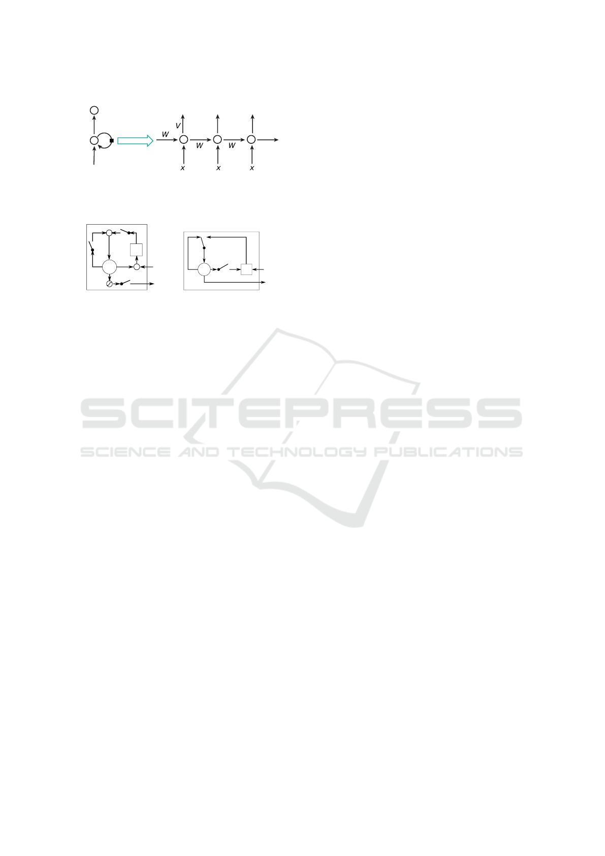
Figure 1: ”A recurrent neural network and the unfolding in

time of the computation involved in its forward computa-

tion.” Image taken from (LeCun et al., 2015).

OUT

(a) LongShort-TermMemory

(b) GatedRecurrent Unit

Figure 2: ”Illustration of (a) LSTM and (b) gated recurrent

units. (a) i, f and o are the input, forget and output gates,

respectively. c and ˜c denote the memory cell and the new

memory cell content. (b) r and z are the reset and update

gates, and h and

h are the activation and the candidate acti-

vation.” Image taken from (Chung et al., 2014).

single instance of an RNN) the amount of information

that can be carried over is subject to a hard theoretical

limit. In practice, of course, NNs are hardly capa-

ble of precisely manipulating every single bit of their

connections, so the practical limit for remembering

past pieces of the input stream must be way below the

inputs vector information memory size.

In this paper, we ﬁrst show that the memorization

of random inputs can in fact be learned by RNNs and

then recognize a hard practical limit to how far a given

RNN architecture can remember the past. We con-

struct the memorization experiment in Section 3). Our

experiments show that a distance limit, i.e., the loss of

the ability to store and reproduce values, occurs very

prominently, of course varying with the type and ar-

chitecture of the RNN (cf. Section 4).

While these experiments explore the basic work-

ings of RNNs, we are not aware of other research as-

sessing a comparable limitation on RNNs. Closest re-

lated work is discussed in Section 5. The existence of

a hard limit in memory distance may have several im-

plications on the design and usage of RNNs in theory

and practice like how big an RNN needs to be so that

it is able to remember the weather from 24 hours ago,

e.g., which we brieﬂy discuss as this paper concludes

(cf. Section 6).

2 FOUNDATIONS

We consider the three most popular types of RNNs for

experiments on their respective memory limits. In this

section, we give a quick recap on their most relevant

properties.

2.1 Recurrent Neural Networks

Recurrent Neural Networks (RNNs) were the ﬁrst

models introduced to process data sets that imply a

temporal dependency on sequential inputs (Schmid-

huber, 2015).

While (given an input vector x = hx

1≤i≤q,i∈N

length q ∈ N) one element x

at a time is processed,

a hidden state vector h carries the history of all the

past elements of the sequence (LeCun et al., 2015).

Finally, a tanh activation function shifts the inter-

nal states to the nodes of the output layer. Given a

sequential input x and an activation function g, the

output state for every time step t is h

= g(Wx

t−1

) (Chung et al., 2014). RNNs can be thought of

as single layer of neural cells, which is reused mul-

tiple times on a sequence while taking track of all

subsequent computations (cp. Figure 1). Therefore,

every position of the output vector z is inﬂuenced by

the combination of every previously evaluated input

as described by:

z = tanh((x wx + b) +(ws  s)) (1)

2.2 Long Short-Term Memory

Networks

While regular RNNs are known for their problems in

understanding long-time dependencies as the gradi-

ent either explodes or vanishes (LeCun et al., 2015;

Chung et al., 2014; Schmidhuber, 2015), Hochre-

iter and Schmidhuber introduced the Long Short-Term

Memory (LSTM) unit (Hochreiter and Schmidhuber,

1997). The main difference lies in the ”connec-

tion to itself at the next time step through a mem-

ory cell” (LeCun et al., 2015) as well as a forget

gate, that regulates the temporal connection (cp. Fig-

ure 2, a). Layers equipped with LSTM cells can learn

what to forget while remembering valuable inputs in

long temporal sequences. However, this functionality

comes at a high computational cost in total trainable

parameters N = 4 ·(mn +n

+ n) where m is the input

dimension, and n is the cell dimension. This consti-

tutes a four-fold increase in comparison to a RNN (Lu

and Salem, 2017).

Empirical Analysis of Limits for Memory Distance in Recurrent Neural Networks

309

2.3 Gated Recurrent Unit Networks

Cho et al. proposed a new LSTM variant, Gated Re-

current Unit (GRU) with reduced parameters and no

memory cell. At ﬁrst ”the reset gate r decides whether

the previous hidden state is ignored”, then ”the up-

date gate z selects whether the hidden state is to be

updated”. In combination with the exposure of the

hidden state, the internal decision gates could be re-

duced from four to ”only two gating units”, so that the

overall number of trainable parameters per layer acti-

vation decreases (see (Cho et al., 2014; Chung et al.,

2014); cp. Figure 2, a). In short, a GRU cell is a hid-

den layer unit that ”includes a reset gate and an update

gate that adaptively control how much each hidden

unit remembers or forgets while reading/generating a

sequence” (Cho et al., 2014). Even though (Chung

et al., 2014) did not prefer GRU over LSTM in an em-

pirical testing setup, they saw that the usage ”may de-

pend heavily on the dataset and corresponding task”.

2.4 Echo State Networks

Echo state networks (ESNs) are a type of reser-

voir computer, independently developed by Herbert

Jaeger (Jaeger, 2001) and Wolfgang Maass (Maass

et al., 2002). Reservoir computing is a framework

which generalises many neural network architectures

utilising recurrent units. ESNs differ from ”vanilla”

RNNs in that the neurons are sparsely connected

(typically around 1% connectivity) and the reservoir

weights are ﬁxed. Also, connections from the input

neurons to the output as well as looping connections

in the reservoir (hidden layer) are allowed, see Fig-

ure 3.

Figure 3: An ESN with all possible kinds of connections.

The legend denotes which ones are ﬁxed, trainable and op-

tional.

Unlike most recurrent architectures in use today,

ESNs are not trained via backpropagation though

time (BPTT), but simple linear regression on the

weights to the output units. Having ﬁxed reservoir

weights makes the initialization even more important.

Well initialized ESNs display the echo state property,

which guarantees, after an initial transient, that the

activation state is a function of the input history:

= E(..., x

t−1

, x

) (2)

Here, E denotes an echo function E = (e

, ..., e

) with

: U

−N

→ R being the echo function of the i-th unit.

Several conditions for echo states have been pro-

posed, the most well-known stating that the spectral

radius and norm of the reservoir matrix must be below

unity (Jaeger, 2001). This has been shown to neither

be sufﬁcient nor necessary (Yildiz et al., 2012; Mayer,

2017), but remains a good rule of thumb.

The amount of information from past inputs that

can be stored in the ESNs transient state dynamics

is often called its short-term memory and is typically

measured by the memory capacity (MC), proposed by

Jaeger (Jaeger, 2001). It is deﬁned by the coefﬁcient

of correlation between input and output, summed over

all time delays

MC =

∞

∑

k=1

∞

∑

k=1

cov

(x(t − k), y

(t))

Var(x(t)) ∗Var(y

(t))

(3)

and thus, measures how much of the inputs variance

can be recovered by optimally trained output units. It

has been shown by Jaeger that the MC of an ESN with

linear output units is bounded above by its number of

reservoir neurons N.

ESNs predate the deep learning revolution.

Nonetheless, deep variants of ESNs have recently

been proposed (Gallicchio and Micheli, 2017) to

make use of the advantages of layering. Reservoir

computing is an active ﬁeld of research, as the models

are less expensive to train, often biologically plausi-

ble (Buonomano and Merzenich, 1995) and allow for

precise description of state dynamic properties due to

the ﬁxed weights of the reservoir.

3 METHODOLOGY

To reveal the limits of distance in which information

can be carried over from past states h

t−n

through re-

current connections of RNN type networks, we con-

struct a task in which the RNN is forced to remember

a speciﬁc input of the input data stream x.

This implies that there must not be any correla-

tion between the pieces of the input data stream so

that there is no way to reconstruct past pieces with-

out fully passing in their values through the recurrent

connections to all future applications of the RNN. We

implemented this experiment using random-length se-

quences of random numbers as input data to the RNN.

ICAART 2022 - 14th International Conference on Agents and Artiﬁcial Intelligence

310

The task (cf. Def. 1) is the reproduction of the pth-

from-last input throughout a training setup for a set

p ∈ N.

However, since the sequences are of random

lengths, the RNN cannot recognize which piece of

the input stream will be needed until the very last ap-

plication. This forces the RNN to carry over all the

information it can from the input stream. We argue

that this is the canonical experiment to test memo-

rization abilities of RNNs. This task deﬁnitions are in

stark contrast to common applications of RNNs where

one explicitly expects some correlations between the

pieces of the input sequence and thus uses RNNs to

approximate a model of said connections.

Deﬁnition 1 (Random Memorization Task). Let q be

a random number uniformly sampled from [10;15] ⊆

N. Let x = hx

1≤i≤q,i∈N

be a sequence of random

numbers x

each uniformly sampled from [0;1] ⊆ R.

Let R be an RNN that is applied to the sequence x

in order with the result R (x) of the last application.

The memorization task of the pth-from-last position

is given by the minimizing goal function f

(R , x) =

q+1−p

− R (x)|.

Note that the random length of the sequence is

substantial. Otherwise, an RNN trained to reproduce

the pth-from-last position may count the position of

the pieces of the input sequence from the start, mak-

ing it rather easy to remember the qth-from-last (i.e.,

ﬁrst) position. In complexity terms, this task requires

space complexity of O(1). These claims are supported

by our experiments in Section 4, where we also test a

ﬁxed-length memorization task:

Deﬁnition 2 (Fixed-Length Random Memorization

Task). Let q = 10. For all else, refer to Def. 1.

4 EXPERIMENTAL RESULTS

To evaluate the task described in Deﬁnitions 1 we

conducted several experiments with different conﬁgu-

rations of RNNs, LSTMs, and GRUs. A conﬁguration

is speciﬁed by the number of layers l of the network

and the number of cells per layer c. We disregarded

any complex architectural pattern by just examining

standard fully connected recurrent layers as well as

modern network training techniques such as gradient

clipping or weight decay in favor of comparability.

Layers’ outputs from more than c ≥ 1 cells are added

up. Weight updates are applied by stochastic gradient

descent (SGD) and the truncated backpropagation al-

gorithm. Training data is generated by sampling from

a Mersenne Twister pseudo-random number genera-

tor. Every network conﬁguration was trained for up to

5000 epochs for 5 different random seeds if not stated

otherwise.

Random Memorization We start by evaluating the

random memorization task (cf. Deﬁnition 1). We

run a simple scenario with l = 1 layer and c = 5

cells within that layer. We conducted 10 indepen-

dent training runs each for every position to memo-

rize from ”position -1”, i.e., the last position or p = 1,

to ”position -10”, i.e., the 10th-from-last position or

p = 10. Figure 4 shows the results for an RNN plot-

ting the loss over training time: Reproducing posi-

tions 1 ≤ p ≤ 4 is learned quickly so that most runs

overlap at the bottom of the plot. p = 5 seems to be

harder to learn as some runs take distinctively more

time to reach a loss close to zero, but the 5th-from-

last random memorization task is still learned reliably.

Positions 6 ≤ p ≤ 8 seem to stagnate not being able to

reduce the loss beyond around 0.15, which still means

that some information about these positions’ original

value is being passed on, though. However, the net-

work greatly loses accuracy and cannot reliably repro-

duce the values. We observe another case in most runs

of positions p = 9 and p = 10, where the loss seems

to stagnate at around 0.25: Note that for the random

memorization task of sequence values x

∈ [0; 1] ⊆ R a

static network without any memorization can simply

always predict the ﬁxed value R (x) = 0.5 to achieve

an average loss of 0.25 on a sequence of random num-

bers. At least, that trick is easily learned by all setups

of RNNs.

We compare those results to experiments executed

for LSTMs in Figure 5. First, we notice that the

LSTM takes much longer training time for the simpler

positions 1 ≤ p ≤ 5, which are all learned eventually

but show a clear separation. This result is intuitive

considering the additional number of weights (total

size 4 ·(mn + n

+ n) for m input elements and n neu-

rons), i.e., trainable parameters, for the same size of

network compared to RNNs (total size mn + n

+ n).

On the other hand, we can observe that LSTMs still

show some learning progress on all positions p after

the 500 epochs plotted here, especially having a run

of position p = 6 taking off towards near-optimal loss.

Thus, there is reason to believe that LSTMs may even-

tually prove to be considerably more powerful than

RNNs given signiﬁcantly longer training times on our

task.

For a more complete overview of the limits of

performance in the random memorization task we

ran this experiment for different number of layers

l ∈ [1; 5] and cells per layer c ∈ [1; 20] ⊆ N as well

as for the pth-from-last positions p ∈ [1; 20] ⊆ N as

a target. Figure 6 shows the results for RNNs. The

color of the respective dots encoding the average loss

Empirical Analysis of Limits for Memory Distance in Recurrent Neural Networks

311

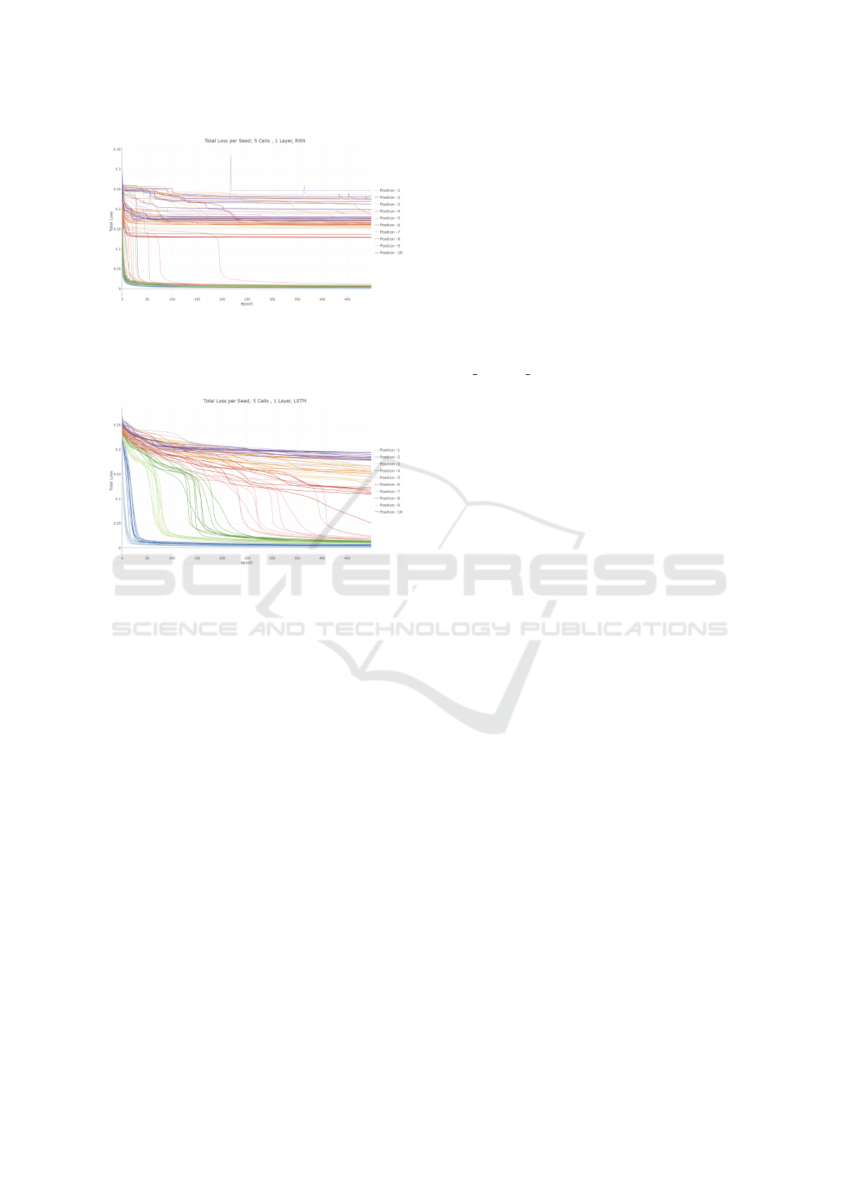
Figure 4: Absolute loss for an RNN with l = 1 layer and c =

5 cells when asked to reproduce the pth-from-last position

(for p ∈ [1; 10]) of a random sequence of random length

q ∈ [10; 15]. Every color shows 10 different training runs

(with different random seed) for a single p.

Figure 5: Absolute loss for an LSTM with l = 1 layer and

c = 5 cells when asked to reproduce the pth-from-last posi-

tion (for p ∈ [1;10]) of a random sequence of random length

q ∈ [10; 15]. Every color shows 10 different training runs

(with different random seed) for a single p.

over 5 independent runs, the scale of the loss is again

ﬁtted to 0.25 as all RNNs manage to learn that ﬁxed

guess as discussed above. We can observe that the

1-layer 1-cell network at the bottom left only learns

to reproduce the last value of the random sequence,

which it can do without any recurrence by just learn-

ing the identity function. It is thus clear why all RNNs

manage to solve this instance. Furthermore, we can

clearly see a monotone increase in difﬁculty when in-

creasing the position, i.e., forcing the network to re-

member more of the sequence’s past. This shows that

no network can learn a generalization of the task that

can memorize arbitrary positions as presumed when

constructing the task.

What is possibly the most interesting result of

these experiments is that the number of instances re-

sulting in average losses of around [0.05;0.2] (colored

in light blue, green) is relatively small: Certain posi-

tions can either be reproduced very clearly or barely

better than the ﬁxed guess (purple, orange), cf. Fig-

ure 7. This implies a strong connection between the

amount of information that can be passed on through-

out the RNN. Furthermore, we can observe that more

cells and more layers (which also bring more cells

to the table) clearly help in solving the memoriza-

tion task. Interestingly, even parallel architectures as

shown for the networks with only one layer (l = 1)

become better with more cells. The connection here

appears almost linear: Within our result data, a one-

layer network with c = n cells can always memorize

the nth-from-last position (p = n) very well.

Figure 8 shows the same experimental setup as de-

scribed above for LSTM networks. In line with the

observation about the loss plots (cf. Figure 5), LSTMs

do not perform as well as RNNs on this task, i.e.,

not satisfyingly solving any position p = 10 instance

(mean absolute loss ≥ 0.04). However, as described

above we conjecture this stems from the fact that the

higher number of weights present in an LSTM net-

work requires substantially longer training times be-

yond what could be performed as part of this experi-

ment. These results still have practical implications:

As this relatively small task consumes large compu-

tational resources, LSTMs seem to be inefﬁcient at

least at (smaller instances of) the random memoriza-

tion task, at least for single layer networks.

We also conducted the same experiments for GRU

networks, as shown in Figure 8. The GRUs’ behav-

ior appears most similar to LSTMs’. We will use

this experiment as a basis to refrain from showing

GRU plots for other experiments since GRUs have

performed that similarly throughout all our experi-

ments. However, note that GRUs require fewer pa-

rameters (N = 3 · (mn + n

+ n)), making them in-

teresting for efﬁcient practical applications (Dey and

Salemt, 2017).

Our results indicate that Jaegers upper bound on

ESN short-term memory remains valid in the context

of deep RNN architectures trained by backpropaga-

tion (RNN, LSTM, GRU). For stacked, multi-layer

architectures, the maximum memory capacity could

not be reached. Instead, we observed an upper bound

of MC ≤ N − (l − 1) with N = c ∗ l.

4.1 Fixed-length Random

Memorization

We now quickly discuss the scenario of Deﬁnition 2:

In this case, we ﬁx the length of the random sequence

q = 10. This means that in theory it is possible to

”count” the positions from the start and thus know

exactly when the currently processed piece of the in-

put data stream needs to be memorized, sparing the

effort of memorizing as many of them as possible un-

til the end. We thus consider this task strictly easier

and our experimental results shown in Figure 9 sup-

ICAART 2022 - 14th International Conference on Agents and Artiﬁcial Intelligence

312

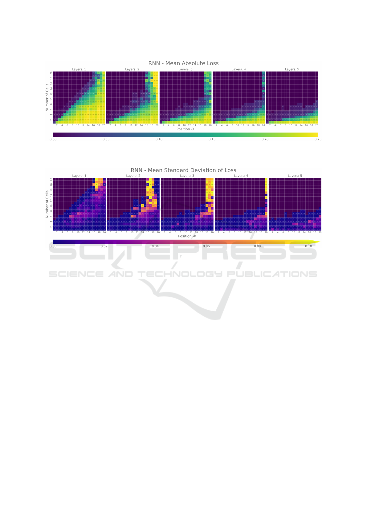
Figure 6: Mean absolute loss for various conﬁgurations of RNNs with l ∈ [1;5] layers with c ∈ [1; 20] cells each when asked

to reproduce the pth-from-last position (for p ∈ [1; 20]) of a random sequence of random length q ∈ [10; 15]. Every data point

is averaged over 5 runs.

Figure 7: Standard Deviation for various conﬁgurations of RNNs with l ∈ [1;5] layers with c ∈ [1; 20] cells each when asked

to reproduce the pth-from-last position (for p ∈ [1; 20]) of a random sequence of random length q ∈ [10; 15]. Every data point

is averaged over 5 runs.

port this. However, the strategy of ”counting from

the start” seems to be subject to some memory limita-

tions as well. Thus, while every instance that is eas-

ily learned in the case of variable-length sequences

is also learnable in this scenario, further learnable in-

stances appear from the right of the plot, i.e., p = 10

for the 1-layer 2-cells network and p ≥ 8 for the 2-

layers 2-cells-each network. This shows that the RNN

is not exactly able to count through the sequence it

is given but able to memorize pieces from the start,

within a similar limit as from the end of the sequence.

As LSTMs and GRUs show a similar behavior, we

omit the respective plots for brevity.

5 RELATED WORK

Recent studies on recurrent neural networks mostly

focused on memory afforded by attractor dynamics

or weight changes while learning. Both are only use-

ful in the context of temporally correlated data, as the

model settling in a low dimensional state space would

not be desirable when every data point is equally im-

portant. As RNNs have been conceived precisely to

recognize and model dependencies in sequential data,

their ability to deal with i.i.d. or uncorrelated input

might seem to be of little importance. We argue that

this capability is an integral part of RNN memory and

performance, which has long been recognized in the

reservoir computing literature. For tasks where the

output should depend strongly on the whole input his-

tory, we require a unique, clearly distinguishable hid-

den state for every input. Using uncorrelated data,

we can approximate the total amount of information

the architecture can store in its transient activation dy-

namics.

In addition, and speciﬁc to RNN-architectures a

lot of empirical evaluations on various LSTM and

RNN conﬁgurations and tasks already exist. Hochre-

iter and Schmidhuber for example evaluated LSTM

cells from the beginning. They conjectured that

gradient-based approaches suffer from practical in-

ability to precisely count discrete time steps and

therefore assume the need for an additional count-

ing mechanism (Hochreiter and Schmidhuber, 1997).

However, our experiments show that an explicit

counting mechanism might not be necessary, even

Empirical Analysis of Limits for Memory Distance in Recurrent Neural Networks

313

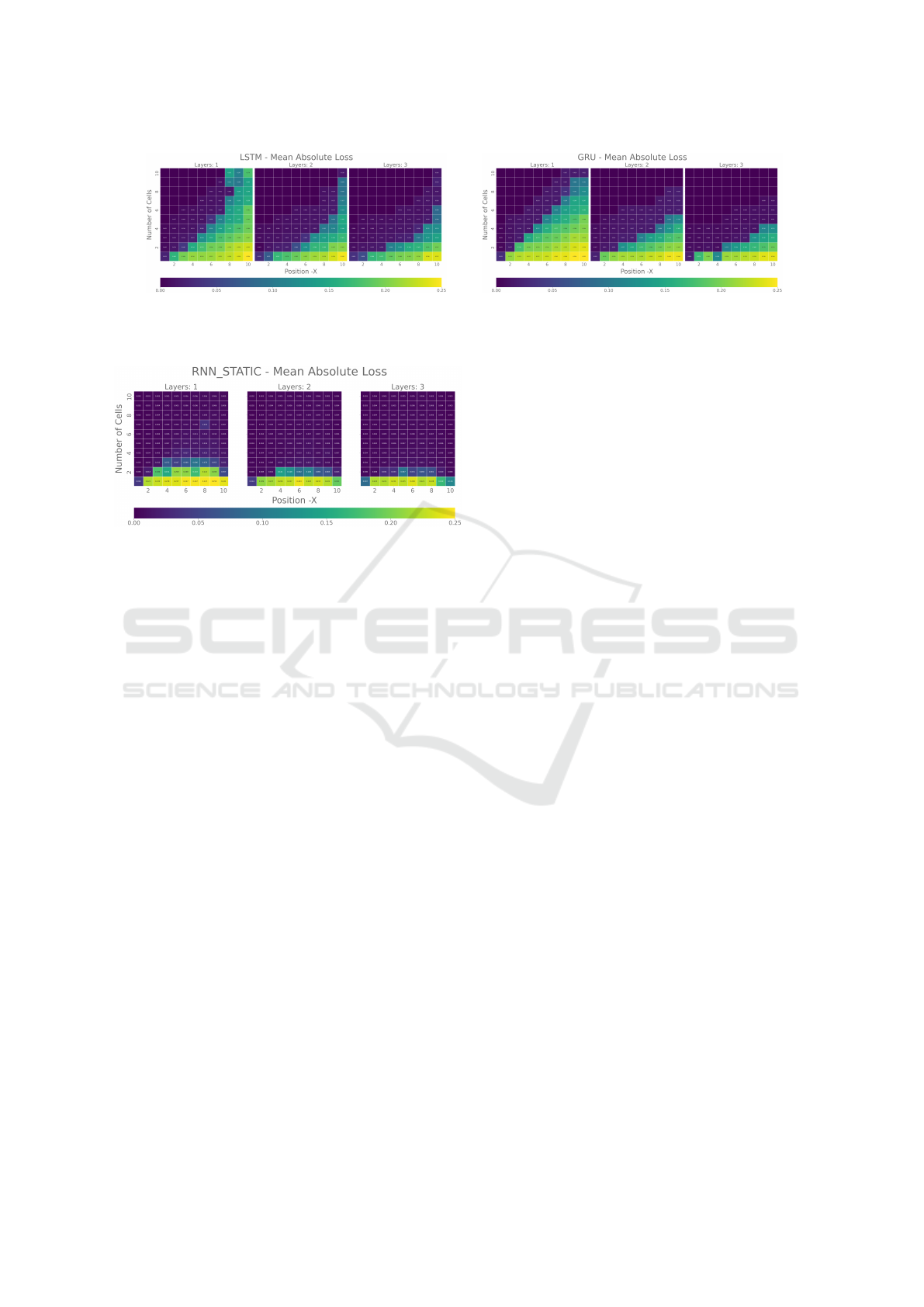
Figure 8: Mean absolute loss for various conﬁgurations of LSTMs (left) and GRU (right) with l ∈ {1, 2, 3} layers with

c ∈ [1; 10] cells each when asked to reproduce the pth-from-last position (for p ∈ [1; 10]) of a random sequence of random

length q ∈ [10; 15]. Every data point is averaged over 10 runs.

Figure 9: Mean absolute loss for various conﬁgurations of

RNNs with l ∈ {1, 2, 3} layers with c ∈ [1; 10] cells each

when asked to reproduce the pth-from-last position (for p ∈

[1;10]) of a random sequence of ﬁxed length q = 10. Every

data point is averaged over 10 runs.

for models, trained on random sequences (i.e., pure

noise). At least for the extend of our observations.

First experiments on the ability of an RNN to carry

information over some distance in the input sequence

were conducted (Cleeremans et al., 1989). Liken-

ing an RNN to a ﬁnite state automaton (for more

details on that line of thought (Giles et al., 1992)),

they trained a network to recognise an arbitrary but

ﬁxed regular grammar. Interestingly, they concluded

that a recurrent network can encode information about

long-distance contingencies only as long as informa-

tion about critical past events is relevant at each time

step, which again contrasts our results on random se-

quences.

Little research has been performed on random se-

quences of variable length as inputs for RNNs. One

could argue that experiments 4 and 5 by Hochreiter

and Schmidhuber are of relevance here (Hochreiter

and Schmidhuber, 1997). However, we like to stress

that our work is focused on random sequences both in

length and value to reproduce an element x

on a spe-

ciﬁc position without providing any form of hint such

as additional labelling or encoding. We see our work

in contrast to these early experiments, as we test for

maximal signal remoteness for a given computational

budget and not necessary for memory endurance in

general. In other words, given an input vector of ran-

domly generated length, they ask for the binary an-

swer to whether a speciﬁc symbol came before an-

other. This tests if the gradient can uphold for enough

recurrent steps so that the two bits of information can

be recognized. In contrast, given a random input vec-

tor of randomly generated length, we ask the networks

to reproduce the pth-last entry. We also considered

classic RNNs that do not possess gated memory vec-

tors.

Most recently Gonon et al. analysed the mem-

ory and forecasting capacities of linear and nonlin-

ear RNN (for independent and non-independent in-

puts). They stated an upper bound for both while

generalizing Jaegers statements regarding MC esti-

mates. (Gonon et al., 2020)

Additionally, Bengio et al. performed related ex-

periments to investigate the problem of vanishing and

exploding gradients. Furthermore, their ﬁndings ex-

plain how robust the transport of information is un-

der the inﬂuence of noisy and unrelated information.

However, they did not consider pure memorization

”by heart”. (Bengio et al., 1994)

As one might confuse the benchmark problems

in this paper with work on the topic of generaliza-

tion and over-ﬁtting, we would like to point out, that

our targeted notion of capacity is very different. Al-

though unrelated in methodology (they used regular

fully connected feed-forward networks), Zhang et al.

provide an analysis quite similar in wording: They

consider a network’s capacity as the amount of input-

output pairs from the training set that can be exactly

reproduced by the network (after training) (Zhang

et al., 2016). This kind capacity is measured on a

whole data set of input vectors. We consider memory

capacity within a single call of a trained network for

a single input vector that is passed in piece by piece,

which is an entirely different setup.

Neural Turing Machines currently are a promis-

ing extension of classical NNs designed speciﬁcally

to offer more powerful operations to manage a hidden

state ((Graves et al., 2014)). We reckon that the Ran-

dom Memorization Task is trivial to them. The same

applies for neural networks architectures that involve

ICAART 2022 - 14th International Conference on Agents and Artiﬁcial Intelligence

314

attention mechanism, like the very prominent Trans-

former (Vaswani et al., 2017).

6 CONCLUSION

We deﬁned the Random Memorization Task for

RNNs. Despite it contradicting the intuition be-

hind the usage of recurrent neural networks, classical

RNNs, LSTM and GRU networks were able to mem-

orize a random input sequence to a certain extent,

depending on conﬁguration and architecture. There

is a discernible borderline between past positions in

the sequence that could be memorized and those that

could not, which correlates with the MC formulated

by Jaeger. We therefor conclude, that Jaegers MC for-

mula is applicable for calculating the memory limit in

respect to the RNN’s type and architecture.

While our experiments are very limited in scale

(due to the already computationally expensive nature

of the experiments), we observe the trend that more

cells increase the memory limit. The limiting fac-

tor that we observed, at least for vanilla-RNN’s, is

the VEGP. However, it is important to note that for

current RNN applications the ratio of input sequence

length and cells inside the RNN is usually in favor

of the number of cells, so that we would not expect

the memory limit to play an important role in the ap-

plication of the typical RNN. Still, we hope this re-

search represents an additional step towards a theo-

retical framework concerned with the learnability of

problems using speciﬁc machine learning techniques.

REFERENCES

Bengio, Y., Simard, P., Frasconi, P., et al. (1994). Learning

long-term dependencies with gradient descent is difﬁ-

cult. IEEE transactions on neural networks, 5(2):157–

166.

Buonomano, D. V. and Merzenich, M. M. (1995). Tem-

poral information transformed into a spatial code by

a neural network with realistic properties. Science,

267(5200):1028–1030.

Cho, K., Van Merri

enboer, B., Gulcehre, C., Bahdanau, D.,

Bougares, F., Schwenk, H., and Bengio, Y. (2014).

Learning phrase representations using RNN encoder-

decoder for statistical machine translation. arXiv

preprint arXiv:1406.1078.

Chung, J., Gulcehre, C., Cho, K., and Bengio, Y.

(2014). Empirical evaluation of gated recurrent neu-

ral networks on sequence modeling. arXiv preprint

arXiv:1412.3555.

Cleeremans, A., Servan-Schreiber, D., and McClelland,

J. L. (1989). Finite state automata and simple recur-

rent networks. Neural computation, 1(3):372–381.

Dey, R. and Salemt, F. M. (2017). Gate-variants of gated

recurrent unit (GRU) neural networks. In 2017 IEEE

60th International Midwest Symposium on Circuits

and Systems (MWSCAS), pages 1597–1600. IEEE.

Engelbrecht, A. P. (2007). Computational intelligence: an

introduction. John Wiley & Sons.

Gallicchio, C. and Micheli, A. (2017). Deep echo state

network (deepesn): A brief survey. arXiv preprint

arXiv:1712.04323.

Giles, C. L., Miller, C. B., Chen, D., Chen, H.-H., Sun,

G.-Z., and Lee, Y.-C. (1992). Learning and extract-

ing ﬁnite state automata with second-order recurrent

neural networks. Neural Computation, 4(3):393–405.

Gonon, L., Grigoryeva, L., and Ortega, J.-P. (2020). Mem-

ory and forecasting capacities of nonlinear recur-

rent networks. Physica D: Nonlinear Phenomena,

414:132721.

Graves, A., Wayne, G., and Danihelka, I. (2014). Neural

turing machines. arXiv preprint arXiv:1410.5401.

Hochreiter, S. and Schmidhuber, J. (1997). Long short-term

memory. Neural Computation, 9(8):1735–1780.

Jaeger, H. (2001). The “echo state” approach to analysing

and training recurrent neural networks-with an erra-

tum note. Bonn, Germany: German National Re-

search Center for Information Technology GMD Tech-

nical Report, 148(34):13.

LeCun, Y., Bengio, Y., and Hinton, G. (2015). Deep learn-

ing. Nature, 521(7553):436.

Lu, Y. and Salem, F. M. (2017). Simpliﬁed gating in

long short-term memory (LSTM) recurrent neural

networks. In 2017 IEEE 60th International Mid-

west Symposium on Circuits and Systems (MWSCAS),

pages 1601–1604. IEEE.

Maass, W., Natschl

ager, T., and Markram, H. (2002). Real-

time computing without stable states: A new frame-

work for neural computation based on perturbations.

Neural computation, 14(11):2531–2560.

Mayer, N. M. (2017). Echo state condition at the critical

point. Entropy, 19(1):3.

Rumelhart, D. E., Hinton, G. E., and Williams, R. J. (1986).

Learning representations by back-propagating errors.

nature, 323(6088):533.

Schmidhuber, J. (2015). Deep learning in neural networks:

An overview. Neural networks, 61:85–117.

Stanley, K. O. and Miikkulainen, R. (2002). Evolving neu-

ral networks through augmenting topologies. Evolu-

tionary computation, 10(2):99–127.

Vaswani, A., Shazeer, N., Parmar, N., Uszkoreit, J., Jones,

L., Gomez, A. N., Kaiser, L., and Polosukhin, I.

(2017). Attention is all you need. In NIPS.

Yildiz, I. B., Jaeger, H., and Kiebel, S. J. (2012). Re-visiting

the echo state property. Neural networks, 35:1–9.

Zhang, C., Bengio, S., Hardt, M., Recht, B., and Vinyals, O.

(2016). Understanding deep learning requires rethink-

ing generalization. arXiv preprint arXiv:1611.03530.

Empirical Analysis of Limits for Memory Distance in Recurrent Neural Networks

315