Estimating the Time-To-Compromise of Exploiting Industrial Control
System Vulnerabilities
Engla Rencelj Ling
a
and Mathias Ekstedt
b
Division of Network and Systems Engineering
KTH Royal Institute of Technology, Stockholm, Sweden
Keywords:
Industrial Control System, Time-To-Compromise, Cyber Security, Vulnerabilities.
Abstract:
The metric Time-To-Compromise (TTC) can be used for estimating the time taken for an attacker to com-
promise a component or a system. The TTC helps to identify the most critical attacks, which is useful when
allocating resources for strengthening the cyber security of a system. In this paper we describe our updated
version of the original definition of TTC. The updated version is specifically developed for the Industrial Con-
trol Systems domain. The Industrial Control Systems are essential for our society since they are a big part of
producing, for example, electricity and clean water. Therefore, it is crucial that we keep these systems secure
from cyberattacks. We align the method of estimating the TTC to Industrial Control Systems by updating the
original definition’s parameters and use a vulnerability dataset specific for the domain. The new definition is
evaluated by comparing estimated Time-To-Compromise values for Industrial Control System attack scenarios
to previous research results.
1 INTRODUCTION
In this paper we introduce a method for estimating the
Time-To-Compromise (TTC) of cyber attacks in In-
dustrial Control Systems (ICS). According to the def-
inition by McQueen et. al., TTC is the “time needed
for an attacker to gain some level of privilege p on
some system component i” (McQueen et al., 2006).
The method introduced in this paper can only esti-
mate the TTC of cyber attacks that exploit vulnera-
bilities reported as Common Vulnerabilities and Ex-
posures (CVEs). It is helpful to estimate the TTC
when creating threat models to assess the cyber se-
curity of systems since the TTC may indicate where
the system is the most vulnerable. If an attack has a
low TTC, one should add measures to protect against
that attack. With TTC, we can also indicate how long
it would take for an attacker to walk an entire path
which allows for proactive planning of cyber security
countermeasures.
The ICS domain is at an increased risk for cy-
ber attacks since our society is vulnerable to a loss
of critical infrastructures, such as, electricity. To en-
sure confidentiality, integrity and availability of ICS,
the systems often have high security requirements and
a
https://orcid.org/0000-0002-9546-9463
b
https://orcid.org/0000-0003-3922-9606
generally have a longer life-cycle of its components.
Also, the reported number of vulnerabilities in ICS
have grown rapidly since the first reports in 1997
(Andreeva et al., 2017). This creates the need for
a method of how to assess the cyber security risks
specifically for ICS to anticipate attacks before they
happen to keep the systems secure.
In this paper we adapt the TTC metric by Mc-
Queen et. al. (McQueen et al., 2006) and introduce
TTC
ICS
as an estimator for specifically focusing on
vulnerabilities and attacks in the ICS domain. The
next section explains the related work. The contin-
ued sections give background to this paper, explain
the method of developing TTC
ICS
and give the defini-
tion of TTC
ICS
. Finally, the last sections are evalua-
tion and discussion.
2 RELATED WORK
The definition of Time-To-Compromise used in this
article was first introduced by McQueen et. al.
(McQueen et al., 2006) and further developments
have been made by, for example, Nzoukou et. al.
(Nzoukou et al., 2013), Zieger et. al (Zieger et al.,
2018) as well as Leversage and Byres (Leversage and
Byres, 2008). The work by McQueen et. al. is de-
scribed in Section 3.2 as part of the background for
96
Rencelj Ling, E. and Ekstedt, M.
Estimating the Time-To-Compromise of Exploiting Industrial Control System Vulnerabilities.
DOI: 10.5220/0010817400003120
In Proceedings of the 8th International Conference on Information Systems Security and Privacy (ICISSP 2022), pages 96-107
ISBN: 978-989-758-553-1; ISSN: 2184-4356
Copyright
c
 2022 by SCITEPRESS – Science and Technology Publications, Lda. All rights reserved

this paper. In the work by Nzoukou et. al. the Mean-
Time-To-Compromise (MTTC) is calculated for any
given network based on the existing known vulnera-
bilities in addition to zero-day attacks. The authors
extend the work by McQueen et. al. by assigning
MTTC to exploits and not components with the aim
to be more granular. They also aggregate the MTTC
of the vulnerabilities by using Bayesian networks. In
this way they are able to aggregate the MTTC while
taking the dependency between multiple attack steps
into consideration. Nzoukou et. al. use values to es-
timate the probability that a vulnerability can be suc-
cessfully exploited.
In the work by Zieger et. al. β-TTC is presented,
which extends the work by McQueen et. al. in ad-
dition to fixing some mathematical flaws. In their
work, they separate the TTC based on compromise
type by dividing the vulnerabilities into four separate
TTC values depending on the types confidentiality,
integrity, availability and execution. They also note
that the assets that are affected by a vulnerability are
often described in vulnerability databases. Therefore
one can use a metric of how severe the vulnerability
is, such as the Common Vulnerability Scoring Sys-
tem (CVSS) (FIRST, 2021), to estimate the TTC per
asset. They also add CVSS values to take the exploit
complexity into consideration, similar to the work by
Nzoukou et. al. (Nzoukou et al., 2013).
Leversage and Byres (Leversage and Byres, 2008)
introduce a Mean Time-To-Compromise (MTTC) in-
terval and a method of how to calculate it. The au-
thors use a modified version of the original TTC (Mc-
Queen et al., 2006) where the frequency of reviews of
the access control list (ACL) rules are included. They
also estimate the TTC based on the average number of
vulnerabilities per node within a zone instead of per
component and introduce a concept of skill indicator,
which they use to replace McQueen et. al.’s value of
fraction of vulnerabilities that are exploitable based
on skill level.
There is also related work with a similar objective
to find the time taken or likelihood of a successful
attack in ICS. In the article by Zhang et. al. (Zhang
et al., 2013), ten SCADA attacks are analyzed and
given three different parameters. P is the probability
of the attack occuring in a SCADA system, k is the
value for how easy the attack is to perform and l is the
value for how severe impact of the attack is. Since the
TTC is related to how easy an attack is to perform,
given that an easy attack is faster to perform, TTC is
correlated to k.
Finally, there is also related work looking at as-
signing probability distributions of attacks instead of
TTC (Xiong et al., 2021). One reason for an attack
to have a low probability distribution could be that
the TTC is high and the attacker is therefore more
likely to successfully use another attack. The authors
used different types of information sources to gain
the probability distributions, including vulnerability
databases.
3 BACKGROUND
There is previous research that constitutes the founda-
tion of TTC
ICS
. Firstly, the TTC
ICS
has been aligned
to the ICS domain by using a dataset of ICS vulner-
abilities compiled by Thomas and Chothia (Thomas
and Chothia, 2020). The dataset made it possible to
develop TTC
ICS
since they did the work of compil-
ing ICS specific vulnerabilities and classifying these.
Secondly, the original TTC by McQueen et. al. has
been the basis when creating TTC
ICS
. In this section
we provide background to both the ICS vulnerability
dataset and the original TTC definition.
3.1 Vulnerability Dataset for Industrial
Control Systems
To create a representative TTC metric for ICS, we
use an ICS specific vulnerability dataset (Thomas and
Chothia, 2020). The ICS vulnerability dataset was
compiled with the aim to increase understanding of
ICS vulnerabilities. In the dataset, there are 2740 ICS
specific known vulnerabilities as of 3rd of September
2020
1
, after removing rejected ones, whereas, for in-
stance, the National Vulnerability Database (NVD)
2
has a total number of more than 150,000 vulnerabili-
ties for all domains.
The dataset by Thomas and Chothia enabled us
to make the TTC metric developed in this paper ICS
specific since they not only scraped the vulnerabil-
ities databases for ICS vulnerabilitites but also cat-
egorized the vulnerabilities. From the dataset, we
use the parameters as seen in Table 3 for estimating
the TTC
ICS
. The severity of vulnerability is repre-
sented by a Common Vulnerability Scoring System
(CVSS) value (FIRST, 2021). The CVSS is described
with a CVSS base score. Part of this base score is
the CVSS exploitability sub score. The exploitabil-
ity sub score is calculated by taking the attack vector,
attack complexity, privilege required and user inter-
1
esorics2020-dataset https://github.com/UoB-
RITICS/esorics2020-dataset [Accessed 24 November
2021]
2
National Vulnerability Database https://nvd.nist.gov/
[Accessed 24 November 2021]
Estimating the Time-To-Compromise of Exploiting Industrial Control System Vulnerabilities
97

Table 1: The new categories for vulnerabilities as proposed
by Thomas and Chothia for the ICS vulnerability dataset
(Thomas and Chothia, 2020).
Category
Access Control Privilege Escalation
and Authentication Weaknesses
Default Credentials
Denial of Service and Resource Exhaustion
Exposed Sensitive Data
Memory and Buffer Management
Permissions and Resource
Weak and Broken Cryptography
Web-based Weaknesses
action into consideration. The other part of the CVSS
base score is the impact score, which defines how se-
vere the impact of exploiting the vulnerability would
be. Even though we do not consider impact, but are
more interested in how difficult the attack is to per-
form, we use both the base score and exploitability
score in TTC
ICS
. This is because the CVSS version
2 does not include exploitability scores in the dataset.
The dataset also includes new categories and product
types assigned by the creators of the dataset. They
assigned the vulnerabilities to eight new main cate-
gories. The eight categories, found in Table 1, cover
95% of the vulnerabilities and the remaining vulnera-
bilities are added to a ninth category of Other. They
also assigned product types, such as Sensor and RTU
to the vulnerabilities. A full list of the product types
are in Table 2.
3.2 Time-To-Compromise by McQueen
et. al.
The work in this paper extends the TTC metric as first
presented by McQueen et. al. (McQueen et al., 2006).
Please note that not all of the McQueens original work
has been included in the TTC
ICS
. The choice was
made to base TTC
ICS
on McQueens original TTC de-
spite further developments that have been made since
those developments did not completely align with the
aim of developing an ICS specific TTC. For example,
in the work by Zieger et. al. they solve a mathematical
flaw for a variable that is not included in the TTC
ICS
(Zieger et al., 2018). This variable is the estimated
number of tries required by an attacker to try vulner-
abilities before finding one that they can exploit. In
TTC
ICS
, this is a fixed number as described in Sec-
tion 4, where all of our adaptions are described. The
definition of TTC according to McQueen et. al. is
provided in this section.
In the work by McQueen et. al., the TTC is cal-
culated for a specific component in a system. In their
Table 2: The new product types for vulnerabilities as pro-
posed by Thomas and Chothia for the ICS vulnerability
dataset (Thomas and Chothia, 2020).
Product Type
AC Drive
Access Management System
Actuator
CCTV
Charging Station
Converter
HMI
Inverter
Network Management
Networking
PLC
Power Metering
Protection System
Remote I/O
RTU
RTU Management
SCADA
Serial Server
Smart Grid
work, the TTC is estimated by dividing the calcula-
tion into three processes. Their method is that the
probability for the attacker to be in the different pro-
cesses and the time taken to complete that processes
are calculated individually and then summed up. In
the first process, there is at least one available exploit
and one known vulnerability for the component. In
the second process, there is at least one vulnerabil-
ity but no known exploit available, and the third pro-
cess is the identification of new vulnerabilities and ex-
ploits. The third process runs in parallel to the first
two processes. The TTC is estimated based on the
attacker skill levels, which are novice, beginner, in-
termediate and expert. The TTC decrease as the skill
level increase since, according to McQueen et. al.,
a higher skilled attacker would have more exploits
available to use.
Below is a summary of TTC, for more details we
kindly refer to the original paper. Equation 1 gives
the likelihood for the attacker to be in process 1, P
1
,
and Equation 2 is the time taken to complete process
1, t
1
. Equation 3 and 4 estimates the same for process
2. Equation 5 calculates the time taken to complete
process 3. Considering that we assume process 3 to
run in parallel with process 1 and 2, the probability to
be in process 3 is always 1. Equation 6 combines all
processes to estimate the final TTC.
Process 1 is calculated according to search theory
as used by Major when modeling terrorism risk (Ma-
jor, 2002) and the assumption is made that the avail-
ICISSP 2022 - 8th International Conference on Information Systems Security and Privacy
98

Table 3: Parameters used from the ICS vulnerability dataset (Thomas and Chothia, 2020) for estimating TTC
ICS
.
Parameter Description
cvss_exploitability_score CVSS Exploitability Score
cvss_base_score CVSS Base Score
u_new_cat Category of the CVE as detected by the dataset creators
u_other_cat Details of ”Other” category of the CVE
u_product_type Type of product
u_sys_created ICS advisory creation date
able exploits are uniformly distributed over the vul-
nerabilities. The probability of the attacker to be in
process 1 increases as the number of vulnerabilities
for the component and number of available exploits
increase and the total number of vulnerabilities de-
crease, but will never reach 1.
P
1
= 1 − e
−vm/k
(1)
where v is the number of vulnerabilities for the com-
ponent that existed in the Internet - Categorization
of Attacks Toolkit (ICAT) database, which has since
been replaced by the National Vulnerability Database
(NVD) (NIST, 2021). k is the total number of vulner-
abilities that were available in the same database. m is
the number of exploits available to the hacker based
on skill level. For a novice the value of m is 50 based
on the number of exploits that existed in Metasploit
and that were easy to use. Metasploit is a software
used for performing exploits (Metasploit, 2021). This
value is then exponentially extrapolated for the next
skill levels to be 150, 250 and 450 for beginner, inter-
mediate and expert, respectively.
t
1
= 1 day (2)
where t
1
is defined as 1 working day or 8 hours by
McQueen. They based this value on experiment re-
sults by Jonsson and Olovsson (Jonsson and Olovs-
son, 1997).
P
2
= e
−vm/k
= 1 − P
1
(3)
where P
1
is Equation 1 described above.
t
2
= 5.8 ∗ ET (4)
where ET is the expected number of vulnerabilities
that an attacker would try to find or create an exploit
for. ET is calculated by a formula that takes into con-
sideration variables, such as, the number of vulnera-
bilities for the component. After the attacker is suc-
cessful in finding the vulnerability that they can ex-
ploit, the tries end. The value of 5.8 is the average
time from the vulnerability announcement to when an
exploit is available in days according to a report ref-
erenced by McQueen et. al. This value is used to
estimate the time taken for each of the tries.
t
3
= ((V /AM) − 0.5) ∗ 30.42 + 5.8 (5)
where V/AM is the inverse of the fraction of vul-
nerabilities that are exploitable based on skill level
and the value of 30.42 is the Mean-Time-Between-
Vulnerabilities (MTBV) in days. The inverse of the
fraction of vulnerabilities that are exploitable is used
because for every vulnerability, the attacker would
need on average 1/f vulnerability and exploit pairs to
find one that is usable for them depending on skill
level. McQueen et. al. values of f are 1, 0.55,
0.30, 0.15, starting with the expert and ending with
the novice. The MTBV is multiplied by this scaling
factor and is then divided by half since they consider
that on average the half point of the fault cycle is the
starting point. The reasoning for this may be that half
way through the fault cycle is where the vulnerability
is most likely found.
T = t
1
∗ P
1
+t
2
∗ (1 − P
1
) ∗ (1 − u) + t
3
∗ u ∗ (1 − P
1
)
(6)
where T is the expected time-to-compromise, u = (1-
(AM/V))
v
, which is the probability that Process 2 is
unsuccessful (u=1 if V=0) and AM/V is fraction of
vulnerabilities that are exploitable for a specific skill
level.
As seen in the equations above, the original TTC
depends on readily available exploits as well as the
fraction of vulnerabilities that are exploitable and the
estimated number of tries to exploit based on the at-
tacker’s skill level. There are also several fixed value
parameters.
4 DEVELOPING AND DEFINING
TTC
ICS
In this section the method of developing TTC
ICS
and
its definition is described. Estimating the TTC by di-
viding the equation into three different processes as
in the original TTC has been kept. The TTC method
was developed in 2006 and have several fixed values
based on the research available at that time. The ad-
justments that have been made are outlined in the fol-
lowing subsections. The last subsection includes how
to represent the TTC
ICS
.
Estimating the Time-To-Compromise of Exploiting Industrial Control System Vulnerabilities
99

4.1 Process 1
As seen in Equation 7, process 1 of TTC
ICS
includes
five different parameters. There are two parameters
for the number of vulnerabilities, k and v, as well as
the number of exploits available m. These three pa-
rameters have been updated as described in the fol-
lowing sections. We have also added the parameters
c2 and c3 to add the vulnerabilities CVSS values into
the equation. For vulnerabilities of CVSS version 2,
the average base score is used and for vulnerabilities
of CVSS version 3, the average exploitability score
is used. This is because the vulnerabilities that are
CVSS version 2 do not have an exploitability score in
the dataset we use. For vulnerabilities of version 3,
we use the exploitability score and for the ones with
version 2, we use the base score.
P
1
= 1 − e
−vm/k
,t
1
= 1 ∗ ((10/c2 + 3, 9/c3)2)days
(7)
where v is the total number of vulnerabilities of that
type component for that type attack (Thomas and
Chothia, 2020), m is the number of exploits available
to the hacker based on skill level, k is the total number
of vulnerabilities (Thomas and Chothia, 2020), c2 is
the average CVSS of version 2 vulnerabilities and c3
is the average CVSS of version 3 vulnerabilities.
4.1.1 Number of Vulnerabilities (v and k)
The v parameter is the total number of vulnerabilities
for that specific component and k is the total number
of vulnerabilities found in the database. In TTC
ICS
,
the source of the vulnerability information was up-
dated to be the ICS specific vulnerability dataset as
described in Section 3.1 (Thomas and Chothia, 2020)
for both of these parameters.
The value of v is found by filtering the ICS vul-
nerability database (Thomas and Chothia, 2020) to
find the total number of vulnerabilities for that type
of component and type of attack. The filter is based
on u_new_cat, u_other_cat and u_product_type
as described in Table 3. For example, to find the value
for access control attacks on an HMI, u_new_cat is
filtered by ”Access control” and u_product_type by
”HMI”.
The value of k is 2740 at the time of writing this
article, since that is the total number of vulnerabili-
ties in the dataset used (Thomas and Chothia, 2020)
after removing rejected entries. The average CVSS
value for the vulnerabilities is calculated by taking the
average CVSS value of all the vulnerabilities for the
component and attack category as found in the ICS
vulnerability dataset (Thomas and Chothia, 2020).
4.1.2 Number of Available Exploits (m)
The number of exploits available to the attacker has
been updated in TTC
ICS
since there are many more
exploits now compared to when the original TTC was
developed. In the original TTC, the number of ex-
ploits available for a novice was set to be 50 based on
the number of trivial exploits in Metasploit. The au-
thors then extrapolated exponentially from 50 to get
the values 50 to 450 available exploits depending on
skill level. We decide to mimic the approach of us-
ing Metasploit, since it is still one of the most com-
mon penetration testing tools which includes many
exploits. Metasploit also ranks the exploits accord-
ing to how reliable they are, which allows us to make
assumptions of which exploits would be usable de-
pending on the attacker skill-level (Rapid7, 2020).
One drawback is that the exploits in metasploit are
not ICS specific. There are tools similar to Metasploit
that are ICS specific, but they contain very few ex-
ploits
3
. Another drawback is that few Metasploit ex-
ploits are ICS specific compared to other frameworks
(Ashcraft et al., 2020). But since Metasploit is free
compared to the other two frameworks and is there-
fore considered to deserve extra attention according
to Ashcraft et. al. (Ashcraft et al., 2020). We also ac-
knowledge that there are more than 44 000 exploits
4
that exist and only a few of them are included in
Metasploit where there are at this point in time 2142
exploits for any given domain. A whitepaper showed
that 8% of ICS/OT CVEs had a public exploit in 2020
(Baines, 2021). Considering the 2740 vulnerabilities
in the ICS vulnerability dataset, if we take 8% of these
vulnerabilities, almost 220 public exploits would be
expected to exist for the ICS domain. Considering
that there is, to our knowledge, no data available for
which of the more than 44 000 exploits that are ICS
specific, we use the Metasploit exploits database and
search through it to find the exploits to use in the es-
timation of TTC.
The value m is achieved by looking at the num-
ber of exploits available to the attacker based on skill
level. The number of exploits available depending
on skill level is calculated based on exploit data from
Metasploit. Using the Metasploit search function, one
can find specific exploit types based on skill level,
called rank by Metasploit. Metasploit divides its ex-
ploits into 7 different ranks depending on how reliable
they are to perform (Rapid7, 2020). We assume that
an expert attacker can perform all exploits because of
their high skill level, but a novice can only perform
3
https://github.com/w3h/isf and
https://github.com/dark-lbp/isf [Accessed 24 Novem-
ber 2021]
4
https://www.exploit-db.com/ [Accessed: 24 November
2021]
ICISSP 2022 - 8th International Conference on Information Systems Security and Privacy
100

exploits with ranking ”Excellent” or ”Great”. Those
exploits are the most reliable and easy to use. For ex-
ample, to find the number of exploits with access con-
trol as part of the description, at skill level excellent,
the following search command is used:
search description:"access control"
type:exploit rank:excellent
The search runs through the module descriptions
since the exploits are not assigned categories of the
type of attack. Because the exploits in Metasploit are
not categorized, the categories assigned in the vulner-
ability dataset can be used as the search terms when
finding exploits in Metasploit. The 7 different ranks
of Metasploit have been divided up based on the 4
different skill levels of TTC
ICS
according to the list
below.
• Expert: Low + Manual + All exploits in Interme-
diate category
• Intermediate: Normal + Average + All exploits in
Beginner category
• Beginner: Good + All exploits in Novice category
• Novice: Excellent + Great
4.1.3 Time to Complete Process 1 ( t
1
)
In the original TTC, the t
1
value was based on experi-
ment results from 1997 where it was suggested that 2
attackers could on average successfully compromise
a component in 4 hours. McQueen et. al. assumed
from those results that it would on average 8 hours or
1 day for one attacker. We chose to update this value
inspired by previous related works.
Similar to the work by Nzoukou et. al (Nzoukou
et al., 2013) and Zieger et. al. (Zieger et al., 2018)
the Common Vulnerability Scoring System (CVSS)
values are included in the method of calculating the
time taken to complete process 1, the variable t
1
. The
CVSS is a framework used to calculate the severity
of vulnerabilities. We add CVSS values so that the
exploitability of the different vulnerabilities is taken
into consideration and not only the quantity of them.
We calculate the average CVSS base score for vulner-
abilities of CVSS version 2, and the average of the
exploitability score for vulnerabilities of CVSS ver-
sion 3, since the CVSS version 2 does not include ex-
ploitability scores. Adding CVSS values also adds
flexibility for the attack abstraction level. For exam-
ple, on the one hand, one can choose to estimate the
TTC for a specific vulnerability and component and
use the specific CVSS for that. On the other hand,
one can combine CVSS values for several vulnerabil-
ities to estimate the TTC for a component based on
the type of attack.
4.2 Process 2
The parameters for estimating the likelihood for an at-
tacker to be in process 2 (P
2
), as seen in Equation 8, is
not described further in this section. The parameters
v, m and k have been described in previous sections.
P
2
= e
−vm/k
= 1 − P
1
(8)
Estimating the time that it would take the attacker
to complete process 2 has been updated and is de-
scribed in the following subsection.
4.2.1 Time to Complete Process 2 (t
2
)
Process 2 is that there is a vulnerability but no read-
ily available exploit. Therefore, the time to complete
process 2 is the time taken to create a new exploit for
a known vulnerability. In the original TTC, this value
is taken from a report published in 2004, but a newer
report shows that the time taken to develop a workable
exploit for a known vulnerability is usually between
6 to 37 days with a median value of 22 days (Ablon
and Bogart, 2017). The report is not ICS specific but
we use this information since we are not aware of any
data stating that the time to develop an exploit is dif-
ferent for the ICS domain compared to any other do-
main. The choice was made to use the range of days
and distribute it based on skill level. Based on the re-
port, we estimate that a novice would take 37 days,
beginner 27 days, intermediate 16 days and expert 6
days by dividing the range uniformly between the four
skill levels.
4.3 Process 3
Since process 3, the identification of new vulnerabil-
ities and developing new exploits, runs in parallel to
the other two processes, we do not estimate the prob-
ability to be in process 3. Regarding the time taken
to complete process 3 there are three parameters to
consider, as seen in Equation 9. One of them is the
time taken to create an exploit for a known vulnera-
bility (t
2
) and the other two are the fraction of vulner-
abilities that are exploitable (f ) and the Mean Time
Between Vulnerabilities (b).
t
3
= ( f
0
− 0.5) ∗ b + t
2
(9)
where t
2
is the number of days taken to develop a new
exploit, f ’ is the inverse of the fraction of vulnerabil-
ities that are exploitable based on skill level and b is
the Mean-Time-Between-Vulnerabilities (MTBV) in
days as calculated from the ICS advisory creation day.
Estimating the Time-To-Compromise of Exploiting Industrial Control System Vulnerabilities
101

Table 4: The number and fraction of vulnerabilities that are exploitable based on skill level.
Skill level CVSS Exploitability Range Exploitable Vulnerabilities
Fraction of Exploitable
Vulnerabilities
Expert 0.1-3.9 1916 1
Intermediate 0.1-3 966 0.50
Beginner 0.1-2.1 455 0.24
Novice 0.1-1.2 105 0.05
4.3.1 The Fraction of Vulnerabilities That Are
Exploitable (f )
In TTC
ICS
the estimated fraction of vulnerabilities
that are exploitable based on skill level is estimated
based on the CVSS exploitability score as found in
the ICS vulnerability dataset (Thomas and Chothia,
2020). The exploitability score instead of the com-
plete CVSS score is used because we are interested
in how many of the vulnerabilities are exploitable and
not in the severity of specific vulnerability. The com-
plete CVSS also includes an estimate of the impact of
exploiting the vulnerability, which we do not consider
as a parameter when estimating the difficulty of per-
forming the exploit. 1916 of the records had the score
assigned from values 0.3 to 3.9. The other records did
not have an assigned score since they are of CVSS
level 2 and for that reason we do not consider those
vulnerabilities. This score is divided into four ranges
based on the different skill levels. We also take into
consideration the theoretical span of the exploitabil-
ity score according to the CVSS calculator (FIRST,
2021), which is 0.1 to 3.9. When estimating the frac-
tion of vulnerabilities that are exploitable, we take
all of the vulnerabilities in the dataset into consider-
ation to gain an overall indication of ICS vulnerabil-
ities that would be exploitable to the skill level. We
assume that a vulnerability with exploitability score
between 0.1 and 1.2 could be exploitable by a novice,
the score 0.1 to 2.1 by a beginner, and so on. Based
on this range, the fraction of vulnerabilities that are
exploitable based on skill level is estimated as seen
in Table 4. The vulnerabilities in the dataset have ex-
ploitability scores of 1.2, 1.8, 2.8 and 3.9. Given the
chosen range, each of these 4 different scores are sep-
arated into 4 different skill levels.
Comparing the values 1, 0.5, 0.24 and 0.05, they
are similar to those used by McQueen et. al., namely
1, 0.55, 0.30, 0.15. In the equation for t
3
the inverse of
the fraction of vulnerabilities that are exploitable are
used according to McQueen et. al.’s original TTC.
4.3.2 Mean-Time Between Vulnerabilities (b)
The value of the Mean-Time Between Vulnerabilities
(MTBV) have been updated based on the ICS advi-
sory disclosure dates of the vulnerabilities (Thomas
and Chothia, 2020). The MTBV is calculated for the
specific scenario when estimating the TTC. But, if the
no vulnerabilities exists in the dataset for the given
scenario, the average number between the disclosures
for all vulnerabilities is used. This was calculated to
be 3.21 days. The MTBV is a difficult value to es-
timate considering, for example, that a study showed
how the related Time Between Vulnerability Disclo-
sure (TBVD) can generally vary over 500% depend-
ing on the product (Johnson et al., 2016). By using
the database, it is possible to first filter out the disclo-
sure dates for a specific product type and then calcu-
late the MTBV. To calculate the MTBV we first sort
the disclosure date to be in order and calculate the
number of days between each date. The average of
these number of days is calculated to find the mean
time between vulnerability disclosure. We make the
assumption that this value is the MTBV since we can-
not know when the vulnerability was found, but only
when it was disclosed.
4.4 The Complete TTC
ICS
The probability of the attacker to be in process 1
and the time taken for the attacker to complete pro-
cesses 1, 2 and 3 are combined and results in the final
TTC
ICS
, as seen in Equation 10.
T = t
1
∗ P
1
+t
2
∗ (1 − P
1
) ∗ (1 − u) + t
3
∗ u ∗ (1 − P
1
)
(10)
where T is the expected time-to-compromise, u = (1-
f)
v
, which is the probability that Process 2 is unsuc-
cessful where v is the number of vulnerabilities and f
is fraction of vulnerabilities that are exploitable for a
specific skill level. Also, u=1 if v=0.
The final TTC
ICS
results in four values of TTC de-
pending on the different attacker skill levels. We sug-
gest that these four values are represented as a proba-
bility distribution since the attacker skill level is most
often unknown. In this way one can estimate the TTC
as a probability distribution which takes the different
skill levels into consideration.
When investigating the best method of how to rep-
resent the TTC
ICS
, different distributions were sur-
ICISSP 2022 - 8th International Conference on Information Systems Security and Privacy
102

Table 5: The categories and product types of the attack scenarios.
Scenario Category Product Type
1 Intrusion in the Substation HMI Access control HMI
2 MITM Attack between Control Center and Substation Information leakage Networking
3 Access to RTU Access control RTU
4 Intrusion in Protective Relay Access control Protection system
5 Malicious Codes in Substation Network Code injection Networking
6 Intrusion through Corporation LAN to Substation LAN Access control Networking
veyed. In the work by Holm (Holm, 2014) it was
shown that the log-normal distribution is the best fit
when modeling the time to compromise of a system
based on analysing data intrusions on computer sys-
tems. They did not, however consider the skill-level
of the attacker. The log-normal distribution was com-
pared to exponential, Weibull, gamma, and the two-
parameter generalized Pareto. On the other hand, the
work by Paulauskas et. al. claims that normal is the
best distribution (Paulauskas and Garsva, 2008). Even
though the classification of attackers is complicated,
the skill level can be divided into 4 levels (Mavroeidis
et al., 2021). We choose to estimate the TTC values
for 4 different skill levels and show the final TTC
ICS
as a log-normal distribution. By doing this we do
not have to consider skill level as a continuous value
during the TTC estimation but instead show the final
probability distribution.
5 EVALUATION
TTC
ICS
is evaluated by comparing the estimated val-
ues to results found in previous research. A discus-
sion for the aptness of this method can be found in
Section 6.
The method of estimating TTC
ICS
is evaluated by
comparing it to the frequency of successful attacks
as calculated by Zhang et. al. (Zhang et al., 2014).
This paper is chosen because their method does not
use CVSS or vulnerability databases. We make the
assumption that an attack that is more frequently suc-
cessful would result in a lower TTC and vice versa.
At the same time, we acknowledge that the TTC of an
attack include more parameters and that the frequency
of success is only one of those factors.
Zhang et. al analyzed six different attack scenar-
ios related to power grids as found in Table 5. The
frequency of success are calculated by using Bayesian
attack graphs where the probability of the attacker to
succeed in each sub-goal of the graph is influenced
by the attacker skill level and potential countermea-
sures. Even though the scenarios include subgoals we
choose to extract the main attack and main compro-
mised component of the scenario to enable a compar-
ison to TTC
ICS
. This is because they only estimate the
frequency of success for the complete scenario. These
main attacks and compromised components can be
found in Table 5 as categories and product types for
each scenario.
The first scenario ”Intrusion in the Substation
HMI” describes how the attacker gains malicious ac-
cess to the substation by scanning the network to iden-
tify the substation and then runs a brute-force or dic-
tionary attack. The attacker then finds the HMI IP
address and access it. We choose to simplify this
scenario to be an access control attack on the HMI
since that is the main attack in the scenario. Scenario
2 ”Man-in-the-Middle (MITM) Attack between Con-
trol Center and Substation” describes how the traffic
between the Control Center and substation is com-
promised by installing an eavesdropper and that false
data is injected. The eavesdropper may have been in-
stalled by exploiting a vulnerability. This scenario we
simplify as information leakage on networking. The
third scenario ”Access to RTU” describes how an at-
tacker can identify a modem (modulation and demod-
ulation) device of the substation and gain access to
the RTU via the modem. This scenario we simplify
as access control on the RTU. The forth scenario ”In-
trusion in Protective Relay” describes how an attacker
can gain malicious access to a protective relay after
the attacker have already gained access to the sub-
station. This scenario we simplify as access control
and for protection system, which is the product type
name used in the ICS vulnerability database. Sce-
nario 5 ”Malicious Codes in Substation Network” ex-
plains how an attacker can inject malicious code into
the substation and we simplify this as code injection
for networking. The last and sixth scenario ”Intru-
sion through Corporation LAN to Substation LAN”
describes how an attacker can attack a substation via
the corporate LAN. We consider this as an access con-
trol attack on networking.
The six different scenarios’ category and product
type from Table 5 are used for estimating the TTC
ICS
.
The first attack scenario is malicious access to the
HMI. To calculate the TTC
ICS
, the ICS vulnerability
dataset is firstly filtered by category ”Access Control”
and product type ”HMI”. There are in total 10 vul-
Estimating the Time-To-Compromise of Exploiting Industrial Control System Vulnerabilities
103

Figure 1: Figure comparing the frequency of successful attacks estimated by Zhang et. al. (Zhang et al., 2014) and estimated
TTC
ICS
for the different scenarios.
nerabilities found, which gives the value of v. Then
the Metasploit exploit database is searched to find the
number of exploits available for an access control at-
tack. The value of RANK depends on the Metasploit
exploit ranking that is described in Section 4. This
resulted in m= 15, 15, 30, 33. The value of k is 2740
as described in the Section 4, which is the total num-
ber of vulnerabilities in the dataset. The Mean Time
Between Vulnerabilties (MTBV) was calculated to be
322 days for product HMI and category of access con-
trol. The average and rounded CVSS value of the ac-
cess control vulnerabilities for HMI is 6,7 for version
2 and 2,6 for version 3. The final TTC
ICS
values are
5, 15, 97 and 3594 days rounded to days for expert,
intermediate, beginner and novice skill levels.
The TTC
ICS
for the next five scenarios were also
estimated so that the difficulty of performing the at-
tacks could be compared to the frequency of success-
ful attacks estimated by Zhang et. al. (Zhang et al.,
2014). They found that the frequency of successful at-
tack was, sorted from high to low, scenario 3, 4, 2, 5, 6
and 1. This means that according to their results, sce-
nario 3 was most frequency successful and scenario
1 the least frequently successful. The higher skilled
attackers always had the highest frequency of suc-
cessful attacks, and the lowest the least. For TTC
ICS
the result was 4, 5, 3, 6, 1 and 2 when comparing
the arithmetic mean, where scenario 4 has the lowest
TTC
ICS
and scenario 2 the highest.
Figure 2 shows the resulting log normal distribu-
tion for the TTC
ICS
of the different scenario as de-
scribed in Zhang et. al. (Zhang et al., 2014). The
log normal distribution is calculated by using the ge-
ometrical mean and standard deviation of the log nor-
mal values for the different scenarios TTC, per skill
level. Most scenarios follow a similar pattern where
the probability of a low TTC value is high, meaning
that the TTC is most likely low. But, there are two
exceptions as seen in Figure 2, which did not exist
for the results by Zhang et. al. (Zhang et al., 2014).
Scenario 4 has a peak in the Probability Distribution
Function (PDF) of around 8 days, indicating that it is
most likely that the TTC of scenario 4 is 8 days rather
than around 1 day for most other scenarios. Scenario
2 has an overall lower PDF for a low TTC, mean-
ing that it is less likely to compromise fast. However,
the probability that it is compromised at all is higher
when the number of days increased. Scenario 4 had
only 3 vulnerabilities in the dataset, with 0 MTBV
and the lowest average CVSS value of the scenarios.
This combined leads to a lower TTC
ICS
value. Sce-
nario 2 had 1 exploit readily available for the attacker
and a MTBV of 265,17. This combined leads to a
higher TTC
ICS
value.
One conclusion that our calculations seems to sug-
gest is that it is easier to successfully gain access
to a protection system than to perform information
leakage on networking equipment. This is also in-
dicated according to an analysis of the U.S. Electric
Sector, ”Strong passwords, authentication, and data
encryption may seem to be obvious measures to em-
ploy when remote access to ICS networks or devices
is necessary, but are often overlooked or ignored.”
(Mission Support Center, 2017). The difficulty of per-
forming an information leakage attack on networking
equipment may be because this equipment is used to
communicate within the ICS and does not transcend
to remote networks. Since the vulnerability dataset
contains vulnerabilities for ICS, it may be true that
information leakage attacks are difficult in ICS net-
working equipment but not in a general IT system.
ICISSP 2022 - 8th International Conference on Information Systems Security and Privacy
104

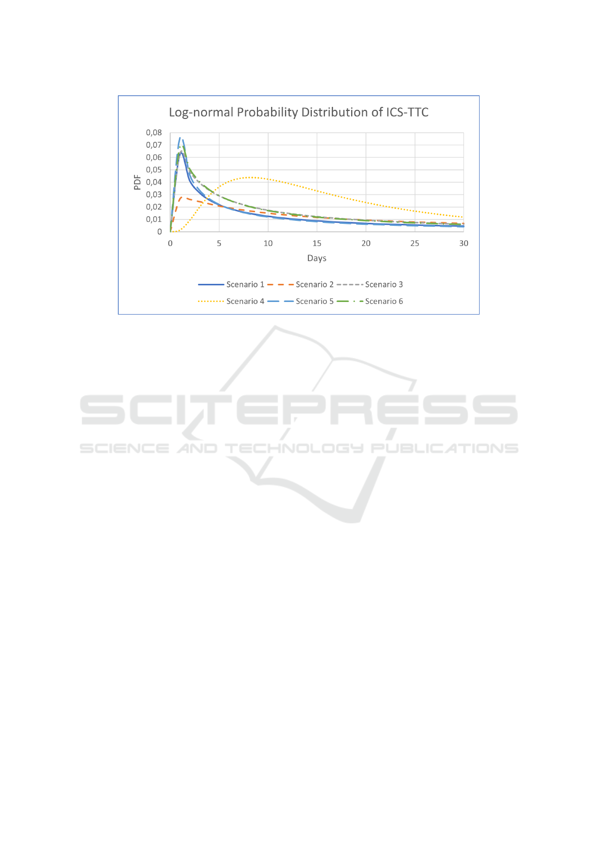
Figure 2: The log-normal probability distribution of TTC
ICS
of the scenario 1-6 for the first 30 days.
6 DISCUSSION
A good method of how to evaluate TTC
ICS
would be
to find the TTC of an attack that has happened in the
past and see if the times are similar. However, it may
be that different attackers would take different amount
of time to perform the same attack. Also, it appears
that it is common for attackers to linger in the envi-
ronment for reconnaissance before the attack is per-
formed (Maynard et al., 2020), which makes it dif-
ficult to know the TTC. Nonetheless, information re-
garding how long attacks take are not readily available
to the best of our knowledge. In the evaluation, we
use information regarding the frequency of successful
attacks instead. We also acknowledge that the sce-
narios of the evaluation combine IT and ICS infras-
tructure. This combination affects the accuracy of the
evaluation since the TTC
ICS
aims to estimate the TTC
specifically in the ICS domain. One potential method
of evaluation could be to observe participants in hack-
ing competitions and track the time it takes for them to
solve the different challenges. Another method could
be to use machine learning and estimating the time
taken for an attack based on a larger dataset. How-
ever, if this larger dataset existed, the machine learn-
ing approach would be a good indication of TTC on
its own.
In this paper, TTC is used as an estimate of like-
lihood and time taken to compromise a component in
the ICS domain. The TTC concept is easy to grasp,
especially in the power systems domain where the
concept Time-To-Failure (TTF) is very familiar. The
TTC is used to estimate the TTC for compromising
vulnerabilities that are found in an ICS vulnerability
dataset (Thomas and Chothia, 2020). We have used
the concept of TTC as defined by McQueen et. al.
(McQueen et al., 2006) and changed it according to
our purpose and by including new research since the
first TTC was developed in 2005.
There are alternatives to estimating which attack
that an attacker is most likely to perform, rather than
looking at the TTC of the attacks. In Threat Model
Quantification (TMQ), they consider which action an
attacker would take based on information regarding
past attacks, interviews with professionals and reports
from attackers describing their end goals (Garcia and
Zonouz, 2014). Our method of estimating TTC is
mostly reliant on information found in databases,
which makes it less subjective but it also raises the
question of the reliability of the dataset used. In the
work by Thomas et. al (Thomas and Chothia, 2020)
the categories and vulnerability detection methods for
the dataset used for TTC
ICS
was validated. The val-
idation was done by assessing the categories on 6
months of new data and by applying the different cate-
gories to vulnerabilities found in a range of ICS prod-
ucts. TTC
ICS
is based on the original TTC so one
should also consider how reliable the original TTC
is. To the best of our knowledge, there is no criti-
cism to the concept of the definition of TTC by Mc-
Queen et. al. There are however criticisms regarding
some specifics to their equation, such as, the parame-
ters used.
It is not possible to estimate the TTC for all types
Estimating the Time-To-Compromise of Exploiting Industrial Control System Vulnerabilities
105

of cyber attacks. For example, the attacks can be
social engineering or bruteforcing attacks. These
types of attacks do not exploit vulnerabilities found in
databases. Using measurements, such as, TTC is also
an oversimplification of the problem with estimating
the probability or time taken for an attack since it it
greatly dependent on the type of attack and to some
extent luck. To acknowledge that the TTC is an esti-
mate and we cannot be certain of an exact TTC, we
suggest representing TTC
ICS
as a log-normal prob-
ability distribution according to the work by Holm
et. al. (Holm, 2014). By representing the estimated
TTC
ICS
values for the different skill levels as a log-
normal probability distribution we are able to add un-
certainty to the result instead of representing it as a
fixed value. We choose to consider zero-day attacks
as part of process 3 because even if an attacker for ex-
ample bought a readily available and previously un-
known exploit, the work to create it would still be es-
timated by process 3. In this way, the estimate would
take both the exploit developer and the exploit ex-
ecutor time into consideration. Parameters that could
potentially be added to calculate TTC is number of
open ports, how often the software is patched, does
the engineers have security training et cetera. We do
not take this parameters into consideration in this arti-
cle but consider these additions as part of future work
since they are related to configurations and the envi-
ronment of specific ICS systems.
Since the TTC
ICS
is reliant on the ICS vulnerabil-
ity dataset (Thomas and Chothia, 2020), future work
includes creating a tool to automatically include infor-
mation from the dataset so that the estimated TTC
ICS
value is dynamic and automatically updates if there
are any changes in the dataset. Regarding the draw-
backs of Metasploit for exploit information, future
work could include a solution to this problem. Some
exploits include the CVE that it exploits, which would
make it possible to match all CVEs in the ICS Vulner-
ability Dataset to all exploits for that CVE and thereby
extracting a list of exploits.
ACKNOWLEDGEMENTS
This research was funded by Swedish Centre for
Smart Grids and Energy Storage (SweGRIDS) and
the centre for Resilient Information and Control Sys-
tems (RICS).
REFERENCES
Ablon, L. and Bogart, A. (2017). Zero Days, Thousands of
Nights: The Life and Times of Zero-Day Vulnerabil-
ities and Their Exploits. RAND Corporation, Santa
Monica, CA.
Andreeva, O., Gordeychik, S., Gritsai, G., Kochetova, O.,
Potseluevskaya, E., Sidorova, S. I., and Timorin,
A. A. (2017). Industrial control systems vulnerabil-
ities statistics. https://media.kasperskycontenthub.
com/wp-content/uploads/sites/43/2016/07/07190426/
KL
REPORT ICS Statistic vulnerabilities.pdf.
Ashcraft, J., Zafra, D. K., and Brubaker, N. (2020).
Threat research. https://www.fireeye.com/blog/threat-
research/2020/03/monitoring-ics-cyber-operation-
tools-and-software-exploit-modules.html.
Baines, J. (2021). Whitepaper: Examining ics/ot exploits:
Findings from more than a decade of data. Technical
report, Dragos, Inc.
FIRST (2021). Common vulnerability scoring system sig.
Garcia, L. and Zonouz, S. (2014). Tmq: Threat model quan-
tification in smart grid critical infrastructures. In 2014
IEEE International Conference on Smart Grid Com-
munications (SmartGridComm), pages 584–589.
Holm, H. (2014). A large-scale study of the time required
to compromise a computer system. IEEE Transactions
on Dependable and Secure Computing, 11(1):2–15.
Johnson, P., Gorton, D., Robert, L., and Ekstedt, M. (2016).
Time between vulnerability disclosures: A measure of
software product vulnerability. Computers & Security,
62.
Jonsson, E. and Olovsson, T. (1997). A quantitative model
of the security intrusion process based on attacker be-
havior. IEEE Transactions on Software Engineering,
23(4):235–245.
Leversage, D. J. and Byres, E. J. (2008). Estimating a sys-
tem’s mean time-to-compromise. IEEE Security Pri-
vacy, 6(1):52–60.
Major, J. (2002). Advanced techniques for modeling terror-
ism risk. The Journal of Risk Finance, 4:15–24.
Mavroeidis, V., Hohimer, R., Casey, T., and Josang, A.
(2021). Threat actor type inference and characteriza-
tion within cyber threat intelligence.
Maynard, P., Mclaughlin, K., and Sezer, S. (2020). De-
composition and sequential-and analysis of known
cyber-attacks on critical infrastructure control sys-
tems. Journal of Cybersecurity, 6.
McQueen, M. A., Boyer, W. F., Flynn, M. A., and Beitel,
G. A. (2006). Time-to-compromise model for cyber
risk reduction estimation. In Gollmann, D., Massacci,
F., and Yautsiukhin, A., editors, Quality of Protection,
pages 49–64, Boston, MA. Springer US.
Metasploit (2021). The world’s most used penetration test-
ing framework.
Mission Support Center, I. N. L. (2017). Cyber
threat and vulnerability analysis of the u.s. elec-
tric sector, mission support center analysis report.
https://www.osti.gov/servlets/purl/1337873.
NIST (2021). General information.
https://nvd.nist.gov/general.
ICISSP 2022 - 8th International Conference on Information Systems Security and Privacy
106

Nzoukou, W., Wang, L., Jajodia, S., and Singhal, A. (2013).
A unified framework for measuring a network’s mean
time-to-compromise. In 2013 IEEE 32nd Interna-
tional Symposium on Reliable Distributed Systems,
pages 215–224.
Paulauskas, N. and Garsva, E. (2008). Attacker skill level
distribution estimation in the system mean time-to-
compromise. In 2008 1st International Conference on
Information Technology, pages 1–4.
Rapid7 (2020). Exploit ranking.
https://github.com/rapid7/metasploit-
framework/wiki/Exploit-Ranking.
Thomas, R. J. and Chothia, T. (2020). Learning from vul-
nerabilities - categorising, understanding and detect-
ing weaknesses in industrial control systems. In Com-
puter Security, Cham. Springer International Publish-
ing.
Xiong, W., Hacks, S., and Robert, L. (2021). A method
for assigning probability distributions in attack simu-
lation languages. Complex Systems Informatics and
Modeling Quarterly, 2021:55–77.
Zhang, Y., Wang, L., and Sun, W. (2013). Investigating
the impact of cyber attacks on power system reliabil-
ity. In 2013 IEEE International Conference on Cy-
ber Technology in Automation, Control and Intelligent
Systems, pages 462–467.
Zhang, Y., Xiang, Y., and Wang, L. (2014). Reliability anal-
ysis of power grids with cyber vulnerability in scada
system. In 2014 IEEE PES General Meeting — Con-
ference Exposition, pages 1–5.
Zieger, A., Freiling, F., and Kossakowski, K. (2018). The
β-time-to-compromise metric for practical cyber secu-
rity risk estimation. In 2018 11th International Con-
ference on IT Security Incident Management IT Foren-
sics (IMF), pages 115–133.
Estimating the Time-To-Compromise of Exploiting Industrial Control System Vulnerabilities
107