
Dynamic Latent Scale for GAN Inversion
Jeongik Cho
a
and Adam Krzyzak
b
Department of Computer Science and Software Engineering, Concordia University, Montreal, Quebec, Canada
Keywords: Generative Adversarial Network, Feature Learning, Representation Learning, GAN Inversion.
Abstract: When the latent random variable of GAN is an i.i.d. random variable, the encoder trained with mean squared
error loss to invert the generator does not converge because the generator loses the information of the latent
random variable. In this paper, we introduce a dynamic latent scale GAN, a method for training a generator
that does not lose the information of the latent random variable, and an encoder that inverts the generator.
Dynamic latent scale GAN dynamically scales each element of the latent random variable during GAN
training to adjust the entropy of the latent random variable. As training progresses, the entropy of the latent
random variable decreases until the generator does not lose the information of the latent random variable,
which enables the encoder trained with squared error loss to converge. The scale of the latent random variable
is approximated by tracing the element-wise variance of the predicted latent random variable from previous
training steps. Since the scale of latent random variable changes dynamically, the encoder should be trained
with the generator during GAN training. The encoder can be integrated with the discriminator, and the loss
for the encoder is added to the generator loss for fast training.
1 INTRODUCTION
The generator of generative adversarial networks
(GAN) (Goodfellow et al., 2014) is trained to map the
latent random variable to the data random variable.
Generally, independent and identically distributed
(i.i.d.) random variable following simple distribution
such as normal or uniform distribution is used as a
latent random variable.
Inverting generator is finding an inverse mapping
of a generator of GAN. It can be used for feature
learning (or representation learning) or various useful
applications such as data manipulation.
There are learning-based methods, optimization-
based methods, and hybrid methods for GAN
inversion. Many methods and applications of GAN
inversion are introduced in the GAN inversion survey
paper (Xia et al., 2021).
Among the learning-based methods, ALI
(Dumoulin et al., 2017), AFL (Donahue et al., 2017),
and BigBiGAN (Donahue et al., 2019) used cGAN
(Mirza et al., 2014) to train an encoder that inverts the
generator. However, those methods are difficult to
train model, and the performance is not good.
a
https://orcid.org/0000-0001-5396-2375
b
https://orcid.org/0000-0003-0766-2659
InfoGAN (Chen et al., 2016), ICGAN (Perarnau
et al., 2016), and Controllable GAN (Zhuang et al.,
2021) used mean squared error (MSE) loss to train the
encoder to recover the latent random variable.
Assuming that the encoder is a gaussian model,
training the encoder with MSE loss is a maximum
likelihood estimation of the encoder (minimize
negative log-likelihood). In-Domain GAN Inversion
(Zhu et al., 2020), and AGEN (Ulyanov et al., 2018)
added reconstruction loss to MSE loss for better
performance. StyleMapGAN (Kim et al., 2021),
Collaborative Learning for Faster StyleGAN
Embedding (Guan et al., 2020), and Encoding in Style
(Richardson et al., 2021) proposed model (StyleGAN
(Karras et al., 2019) and StyleGAN2 (Karras et al.,
2020)) specific methods.
However, using MSE loss to train the encoder
results in a convergence problem because the
generator may lose the information of the latent
random variable. In other words, it is impossible to
train an encoder that inverts the generator trained with
the latent random variable as is because the generator
may ignore some information of the latent random
variable.
Cho, J. and Krzyzak, A.
Dynamic Latent Scale for GAN Inversion.
DOI: 10.5220/0010816800003122
In Proceedings of the 11th International Conference on Pattern Recognition Applications and Methods (ICPRAM 2022), pages 221-228
ISBN: 978-989-758-549-4; ISSN: 2184-4313
Copyright
c
2022 by SCITEPRESS – Science and Technology Publications, Lda. All rights reserved
221

In this paper, we introduce a dynamic latent scale
GAN (DLSGAN), a learning-based method for
training an encoder that inverts the generator of GAN.
DLSGAN dynamically adjusts the scale of the latent
random variable so that the generator does not lose
the information of the latent random variable. This
enables the encoder to converge when training the
encoder with squared error loss (maximum likelihood
estimation).
The scale of the latent random variable depends
on the amount of information that the encoder can
recover. It can be approximated from the element-
wise variance of the predicted latent random variable
from the encoder. DLSGAN traces the predicted
latent codes of past training steps to approximate the
element-wise variance of the predicted latent random
variable.
In DLSGAN, since the scale of a latent random
variable dynamically changes, the encoder should be
trained with a generator during GAN training.
Furthermore, the encoder can be integrated with the
discriminator for efficient training. Also, training the
encoder can be accelerated by adding an encoder loss
to generator loss. It means that the encoder and
generator are trained cooperatively to minimize the
encoder loss. This is possible because the encoder is
trained during the GAN training.
Full codes of our work are available at
“https://github.com/jeongik-jo/DLSGAN”.
2 PROBLEM STATEMENT
Assume that generator maps the latent random
variable to the data random variable (i.e.,
). Our goal is to train an encoder that inverts
the generator (i.e.,
).
When the latent random variable is a
-
dimensional i.i.d. random variable, the encoder can
be considered as an integration of
encoders, where
each encoder is trained to recover each element of a
latent random variable (i.e.,
). Assuming each
encoder is a gaussian model, training each encoder
with an MSE loss minimizes negative log-likelihood
of each encoder.
However, the integrated encoder cannot fully
recover the latent random variable because there is
no guarantee that the generator
uses all the
information of the latent random variable . For
example, when the latent random variable has too
many dimensions, generator can be trained to
ignore some elements of the latent random variable
. Or, generator
can be trained so that some
elements of the latent random variable have
relatively more information than others. In other
words, different latent codes and sampled from
the latent random variable can be mapped to the
same or similar generated data points
and
.
Therefore, some encoders of the integrated encoder
cannot converge to predict some element of the latent
random variable . It means that the generator loses
the information of the latent random variable , and
the encoder cannot perfectly recover the latent
random variable from the generated data random
variable
.
3 DYNAMIC LATENT SCALE
GAN
To prevent the generator from losing information
of the latent random variable , we introduce a
DLSGAN that dynamically adjusts the scale of each
element of the latent random variable .
Assume that the latent random variable is
-
dimensional i.i.d. random variable with the variance
. When the encoder is trained long enough to
predict the latent random variable from the
generated data random variable
with MSE loss,
the variance of each element of the predicted latent
random variable
represents
information of the latent random variable that can
be recovered from the generated data random variable
. If the variance of -th predicted latent random
variable
is zero, it means that the encoder
cannot recover any information of
-th latent random
variable
from the generated data random variable
. On the other hand, if the variance of the -th
predicted latent random variable
is
, then the
encoder can recover all information of
-th latent
random variable
from the generated data random
variable
. Therefore, if the element-wise
variance of the predicted latent random variable
and the element-wise variance of the latent random
variable
are the same, it means that the generator
does not lose the information of the latent random
variable , and the encoder can converge to predict
the latent random variable from the generated data
random variable
.
DLSGAN dynamically adjusts the scale of each
element of latent random variable
according to the
variance of each element of the predicted latent
random variable
so that the element-wise variance
of the latent random variable
and predicted latent
random variable
are equal. Since the dynamic
ICPRAM 2022 - 11th International Conference on Pattern Recognition Applications and Methods
222

latent scale GAN requires both the encoder and the
generator to be trained together during GAN
training, it is efficient to integrate the encoder into
the discriminator . For the same reason, the
generator and the encoder can be trained
cooperatively. That is, encoder loss
can be
added to generator loss
.
The following algorithm shows the process of
obtaining the loss for training DLSGAN.
Algorithm 1: Obtaining loss for training DLSGAN.
function GetLoss(D,G,Z,X,v):
1 z←sample
Z
2 x←sample
X
3 s←
d
z
v
∘1/2
v
∘1/2
2
4 a
g
,z
'
←DG
z∘s
5 L
enc
←avg
z-z
'
∘2
∘s
∘2
6 a
r
,_←D
x
7 L
d
←f
d
a
r
,a
g
+λ
enc
L
enc
8 L
g
←f
g
a
g
+λ
enc
L
enc
9 v←updatev,z
'
∘2
10 return L
d
,L
g
,v
In Algorithm 1, , , , and represent
discriminator, generator, latent random variable, and
data random variable, respectively. Since the encoder
is integrated with the discriminator , the
discriminator outputs two values: 1-dimensional
adversarial value and
-dimensional predicted latent
code. represents the element-wise variance of the
predicted latent random variable
. It is ideal to
approximate the predicted latent variance vector for
every training step, but for efficiency, the predicted
latent variance vector is approximated through
predicted latent codes from the past training steps.
In lines 1 and 2, is a
-dimensional i.i.d. latent
random variable, and is a data random variable. In
Algorithm 1, it is assumed that latent random variable
follows a distribution with a mean of 0 and a
variance of 1 for convenience. is a function
that samples a single sample from a random variable.
represents a latent code, which is sampled from the
latent random variable . represents a data point,
which is sampled from the data random variable .
In lines 3 and 4, is the latent scale vector.
represents the element-wise square root of
the example vector .
represents the L2
norm of example vector
. “” represents element-
wise multiplication.
is the generated data
point with scaled latent code
. In line 4,
represents the adversarial value of generated data, and
represents the predicted latent code, respectively.
When all elements of are the same, i.e., when the
variance of all elements of predicted latent random
variable
are the same, the scaled latent random
variable has the largest differential entropy. On
the other hand, when the variance of only one element
of the predicted latent random variable is not 0, and
the other elements are 0, the scaled latent random
variable has the least differential entropy.
is a constant multiplied to make the scaled latent
random variable equal to the latent random
variable when the differential entropy of the scaled
latent random variable is the largest. The
differential entropy of the scaled latent random
variable dynamically changes according to the
variance of the predicted latent random variable
during GAN training. As GAN training progresses,
the scaled latent random variable converges to
have an optimal entropy representing the real data
random variable through the generator .
In line 5,
represents the element-wise
square of the example vector
. is a function
that calculates the average of a vector.
is encoder
loss. The encoder loss
is equal to the MSE loss
between the scaled latent code and the scaled
predicted latent code
.
In line 6,
represents the adversarial value of a
real data point . “” represents not using value. Since
the latent code of the real data point
is unknown, the
predicted latent code for the real data point
is not
used in DLSGAN training.
In lines 7 and 8,
and
are adversarial loss
functions for discriminator and generator ,
respectively. One can find many adversarial losses in
GAN adversarial losses compare paper (Lucic et al.,
2018).
is encoder loss weight. One can see
encoder loss
is added to both generator loss
and discriminator loss
. This means that the
generator and discriminator are trained
cooperatively to reduce the encoder loss
.
Training the encoder during the GAN training
enables to add encoder loss
to generator loss
.
In line 9, function updates the predicted
latent random variable variance with the new
predicted latent code
. Since the mean of the
predicted latent random variable
becomes
Dynamic Latent Scale for GAN Inversion
223
automatically zero,
(element-wise square of
predicted latent code
) can be considered as the
sample variance of the predicted latent random
variable
. A moving average or an exponential
moving average can be used for the function.
Note that the latent code input to the generator
should always be scaled by the scale vector .
Therefore, the generated data point is
, and
the recovered data point of is
, where
is
the predicted latent code of the real data point .
DLSGAN is still the maximum likelihood
estimation of the encoder (minimize negative log-
likelihood), but the generator
does not lose the
information of the latent random variable , which
allows the encoder to converge when training the
encoder with squared error loss.
4 EXPERIMENT RESULTS AND
DISCUSSION
4.1 Experiment Settings
We trained GAN to generate the CelebA dataset (Liu
et al., 2015) resized to resolution. As the
model architecture, StyleGAN2 with a reduced filter
size of convolution layers was used.
Batch operation (minibatch stddev layer) in the
discriminator and noise in the generator are removed
so that the encoder encodes one data point as one
latent code. As an adversarial loss, NSGAN with R1
regularization (Mescheder et al., 2018) was used as
StyleGAN2. The hyperparameters used for the
experiments are as follows. Most hyperparameters are
the same or similar as StyleGAN2.
Note that optimizer for the mapper of generator
has learning rate as same as StyleGAN2.
is R1 regularization weight. The original paper
introduced R1 regularization used as
regularization weight, so based on that definition, is
20 when
is 10.
We compared the performance of the model with
and without dynamic latent scale. Without dynamic
latent scale means MSE loss was used for encoder
training. We also compared the effect of the encoder
loss
on generator loss
. For the
function for dynamic latent scale, we used a moving
average using the past samples.
The experiments were conducted for i.i.d. latent
random variables with distributions
and
so that the mean and the variance of the
distribution are 0 and 1, respectively.
4.2 Experiment Results
The following figures present the performance results
with and without dynamic latent scale and encoder
loss
on generator loss
or not.
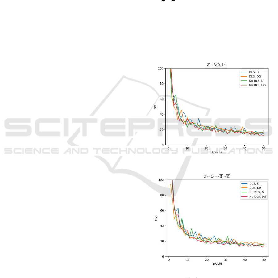
Figure 1: FID comparison when
.
Figure 2: FID comparison when
.
Figures 1 and 2 show the FID (Heusel et al., 2017)
according to the training methods for each epoch. In
figures 1 and 2, “DLS” and “No DLS” represent with
dynamic latent scale and without dynamic latent
ICPRAM 2022 - 11th International Conference on Pattern Recognition Applications and Methods
224
scale, respectively. “D” represents weighted encoder
loss
was added to only discriminator loss
, and “DG” represents weighted encoder loss
was added to both discriminator loss
and
generator loss
. “No DLS, D” corresponds to
previous learning-based methods that do not use a
dynamic latent scale for GAN inversion (e.g.,
ICGAN, Controllable GAN).
One can see that there is little difference in the
generative performance for each training method.
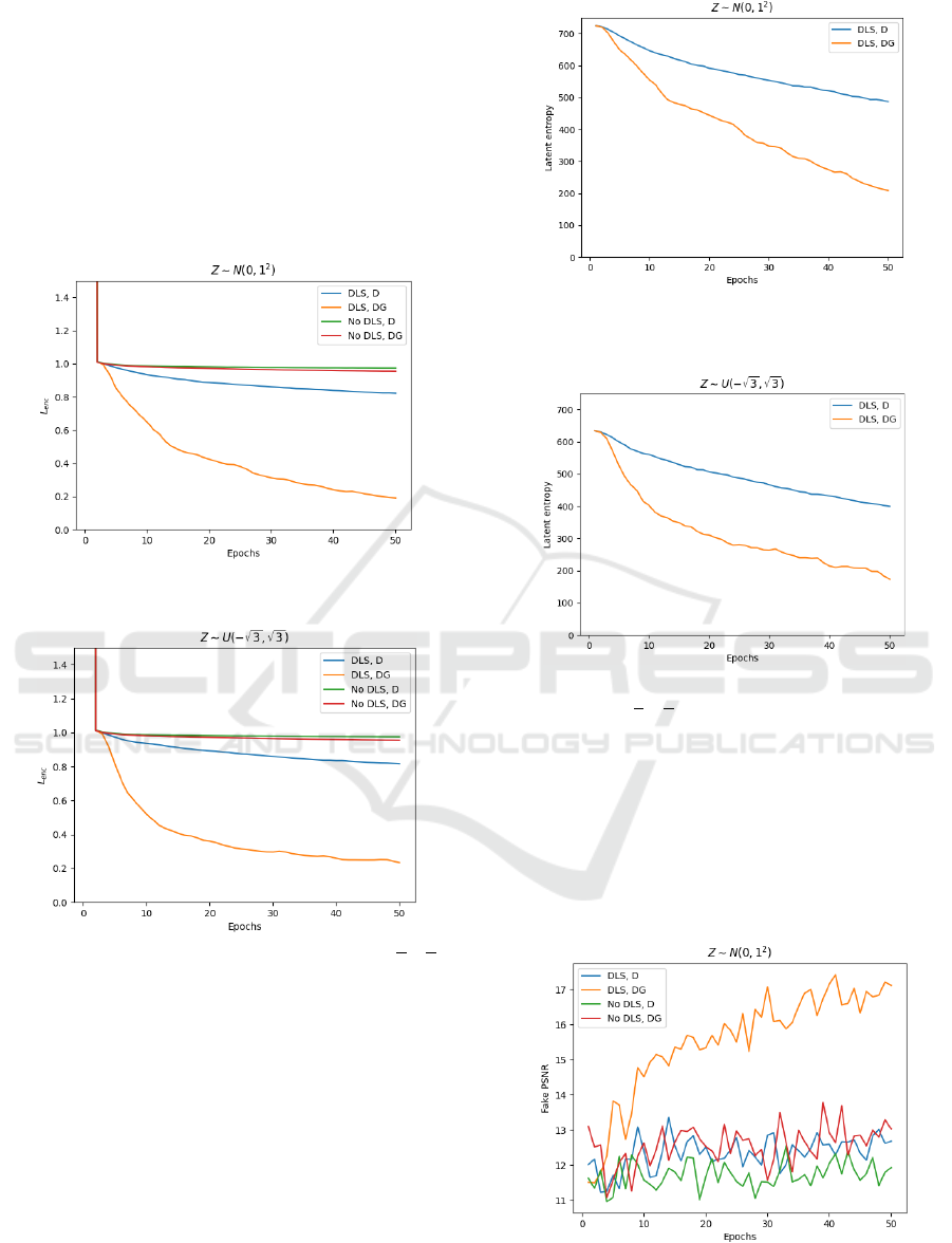
Figure 3: Average
when
Figure 4: Average
when
.
Figures 3 and 4 show the average encoder loss
according to the training methods for each
epoch. One can see that without dynamic latent scale,
encoder loss
hardly changes from 1. This shows
that encoder trained without dynamic latent scale
fails to converge because generator loses
information of latent random variable . On the other
hand, one can see that the encoder loss
continuously decreases as training progresses with
dynamic latent scale. This shows that the model
converges with the dynamic latent scale. Also, one
can see that the encoder loss
is much lower when
encoder loss
is added to the generator loss
.
Figure 5: Differential latent entropy of DLSGAN when
.
Figure 6: Differential latent entropy of DLSGAN when
.
Figures 5 and 6 show differential entropy of
scaled latent random variable with dynamic
latent scale for each epoch. Like encoder loss
,
one can see that the differential entropy of the scaled
latent random variable decreases faster when
encoder loss
is added to the generator loss
.
Note that differential entropy can be negative.
Figure 7: Average PSNR for generated images
reconstruction when
.
Dynamic Latent Scale for GAN Inversion
225
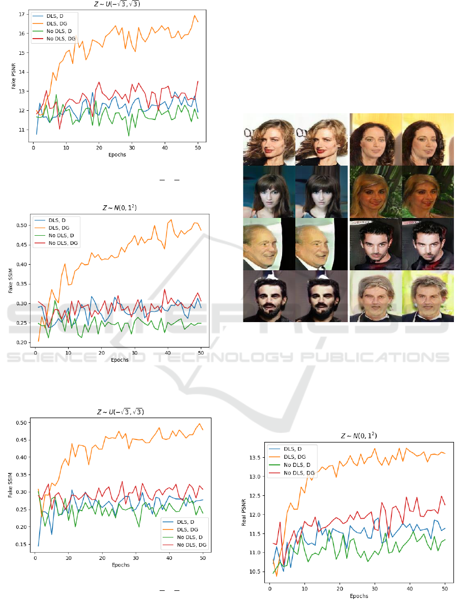
Figure 8: Average PSNR for generated images
reconstruction when
.
Figure 9: Average SSIM for generated images
reconstruction when
.
Figure 10: Average SSIM for generated images
reconstruction when
.
Figures 7-10 show the average PSNR and SSIM
for each epoch when reconstruction is performed on
the generated images. The higher the PSNR and
SSIM, the better the image reconstruction
performance. The PSNR ranges from zero to infinity,
and the SSIM ranges from zero to one. One can see
that the performance of reconstruction on generated
images is much better with DLS, DG. Also, both with
dynamic latent scale and without dynamic latent scale
performed better when the encoder loss
is added
to the generator loss
.
Figure 11: DLS, DG generated images reconstruction
examples when
. Left: generated
image, right: reconstructed image in each image pair.
Figures 11 shows examples of generated images
reconstruction, with dynamic latent scale and encoder
loss
on generator loss
when
.
Figure 12: Average PSNR for test images reconstruction
when
.
ICPRAM 2022 - 11th International Conference on Pattern Recognition Applications and Methods
226
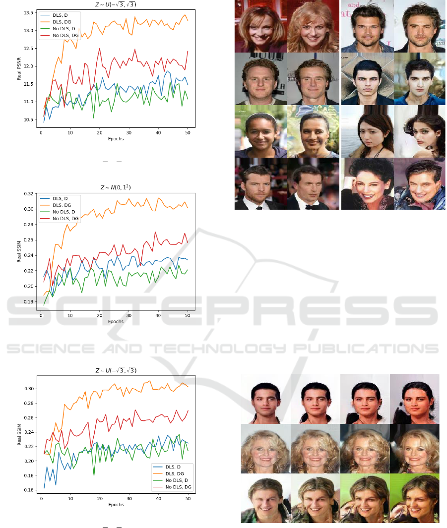
Figure 13: Average PSNR for test images reconstruction
when
.
Figure 14: Average SSIM for test images reconstruction
when
.
Figure 15: Average SSIM for test images reconstruction
when
.
Figures 12-15 show the average PSNR and SSIM
for each epoch when reconstruction is performed on
the test images (real images). One can notice that
reconstruction performance on test images is much
better with DLS, DG.
Figure 16: DLS, DG test images reconstruction examples
when
. Left: test image, right:
reconstructed image in each image pair.
Figures 16 shows examples of generated images
reconstruction with dynamic latent scale and encoder
loss
on generator loss
when
.
4.3 Latent Interpolation of DLSGAN
The following figures show some additional results
with DLS, DG, and
.
Figure 17: Latent interpolation on most important element.
Figures 17 shows interpolating one important
element of the latent random variable from -2 to 2
with DLS, DG, and
. The larger
the elements of the scale vector , the more important
(more informative) elements.
Dynamic Latent Scale for GAN Inversion
227

5 CONCLUSIONS
In this paper, we proposed a DLSGAN, a method for
training a generator that does not lose the information
of the latent random variable, and an encoder that
inverts the generator. Dynamic latent scale GAN
dynamically adjusts the scale of the i.i.d. latent
random variable to have the optimal entropy to
express the data random variable. This ensures that
the generator does not lose the information of the
latent random variable so that the encoder can
converge to invert the generator with maximum
likelihood estimation. The encoder of DLSGAN
showed much better performance than without
dynamic latent scale.
REFERENCES
Goodfellow, I., Pouget-Abadie, J., Mirza, M., Xu, B.,
Warde-Farley, D., Ozair, S., Courville, A., and Bengio,
Y. (2014). Generative Adversarial Nets. In Advances in
Neural Information Processing Systems 27.
Xia, W., Zhang, Y., Yang, Y., Xue, J. H., Zhou, B., and
Yang, M. H. (2021). GAN Inversion: A Survey. arXiv
preprint arXiv:2101.05278.
Dumoulin, V., Belghazi, I., Poole, B., Lamb, A., Arjovsky,
M., Mastropietro, O., and Courville, A. (2017).
Adversarially Learned Inference. In International
Conference on Learning Representations 2017.
Donahue, J., Krähenbühl, P., and Darrell, T. (2017).
Adversarial Feature Learning. In International
Conference on Learning Representations 2017.
Donahue, J., and Simonyan, K. (2019). Large Scale
Adversarial Representation Learning. In International
Conference on Learning Representations 2019.
Mirza, M., Osindero, S. (2014). Conditional Generative
Adversarial Nets. arXiv preprint arXiv:1411.1784.
Chen, X., Duan, Y., Houthooft, R., Schulman, J., Sutskever,
I., and Abbeel, P. (2016). InfoGAN: Interpretable
Representation Learning by Information Maximizing
Generative Adversarial Nets. In Advances in Neural
Information Processing Systems 29.
Perarnau, G., Weijer, J. V. D., Raducanu, B., and Álvarez,
J. M. (2016). Invertible Conditional GANs for image
editing. arXiv preprint arXiv:1611.06355.
Zhuang, P., Koyejo, O. O., and Schwing, A. (2021). Enjoy
Your Editing: Controllable GANs for Image Editing via
Latent Space Navigation. In International Conference
on Learning Representations 2021.
Zhu, J., Shen, Y., Zhao, D., and Zhou, B. (2020). In-domain
GAN Inversion for Real Image Editing. In Proceedings
of European Conference on Computer Vision.
Ulyanov, D., Vedaldi, A., and Lempitsky, V. (2018). It
Takes (Only) Two: Adversarial Generator-Encoder
Networks. Proceedings of the AAAI Conference on
Artificial Intelligence.
Kim, H., Choi, Y., Kim, J., Yoo, S., and Uh, Y. (2021).
Exploiting Spatial Dimensions of Latent in GAN for
Real-Time Image Editing. Conference on Computer
Vision and Pattern Recognition, pages 852-861.
Guan, S., Tai, Y., Ni, B., Zhu, F., Huang, F., Yang, X.
(2020). Collaborative Learning for Faster StyleGAN
Embedding. arXiv preprint arXiv:2007.01758.
Richardson, E., Alaluf, Y., Patashnik, O., Nitzan, Y., Azar,
Y., Shapiro, S., and Cohen-Or, D. (2021). Encoding in
Style: A StyleGAN Encoder for Image-to-Image
Translation. Proceedings of the IEEE/CVF Conference
on Computer Vision and Pattern Recognition, pages
2287-2296.
Karras T., Laine, S., and Aila, T. (2019). A Style-Based
Generator Architecture for Generative Adversarial
Networks. IEEE/CVF Conference on Computer Vision
and Pattern Recognition, pages 4396-4405.
Karras, T., Laine, S., Aittala, M., Hellsten, J., Lehtinen, J.,
and Aila, T. (2020). Analyzing and Improving the
Image Quality of StyleGAN. IEEE/CVF Conference on
Computer Vision and Pattern Recognition, pages 8107-
8116.
Lucic, M., Kurach, K., Michalski, M., Gelly, S., and
Bousquet, O. (2018). Are GANs Created Equal? A
Large-Scale Study. Advances in Neural Information
Processing Systems 31.
Liu, Z., Luo, P., Wang, X., and Tang, X. (2015). Deep
Learning Face Attributes in the Wild. Proceedings of
International Conference on Computer Vision, pages
3730-3738.
Mescheder, M., Nowozin, S., and Geiger, A. (2018). Which
Training Methods for GANs do actually Converge?
Proceedings of the 35th International Conference on
Machine Learning, pages 3481-3490.
Heusel, M., Ramsauer, H., Unterthiner, T., Nessler, B., and
Hochreiter, S. (2017). GANs Trained by a Two Time-
Scale Update Rule Converge to a Local Nash
Equilibrium. Proceedings of the 31st International
Conference on Neural Information Processing System.
ICPRAM 2022 - 11th International Conference on Pattern Recognition Applications and Methods
228
