A Queueing Analysis of Multi-type Servers and Multi-type Customers

System based on Gas Stations

Yoshito Machida

and Tuan Phung-Duc

2 a

Graduate School of Science and Technology, University of Tsukuba, Tsukuba, Ibaraki 305-8577, Japan

Faculty of Engineering, Information and Systems, University of Tsukuba, Tsukuba, Ibaraki 305-8577, Japan

Keywords:

Queueing Model, GI/M/1-type Markov Chain, Gas Station, Performance.

Abstract:

Nowadays, cars are essential to life, and most cars used in society need refueling. In gas stations, an odd

phenomenon often occurs where the server (refueling lane) is available, but the service is not available, and

this is due to the mismatch between the type of the customer (car) and the type of the server. In this paper,

we model some types of the system of gas stations as queueing models and analyze them. In addition, we

derive performance measures and compare these types of systems. Some counter-intuitive results emerge in

this study.

1 INTRODUCTION

Nowadays, many people worldwide use cars, and

transporting by cars is essential for their lives. There

are over 80 million cars in Japan, and over 60 million

are passenger vehicles (Ministry of Land, Infrastruc-

ture, Transport and Tourism, Japan, 2021). Recently,

zero-emission vehicles are developing, such as Elec-

tric Vehicles (EVs) and Fuel Cell Vehicles (FCVs),

but the number of such vehicles is still low. In Japan,

the number of EVs and FCVs is about 130 thousand

at the end of FY (Fiscal Year) 2019 (Next Genera-

tion Vehicle Promotion Center, Japan, 2020). Accord-

ingly, most cars on the streets are powered by engines

which need to be refueled. Generally, people refuel

cars at a Gas Station (GS), and some unusual phe-

nomena occur.

Typically, each refueling machine installed at a

GS has two servers (refueling lanes), and each lane

can provide refueling service independently. Here-

after, we refer the server to as a service lane in a re-

fueling machine. Most cars have a fuel door on either

the left or right side, so the two lanes are for cars with

a left-side fuel door and a right-side fuel door. In real-

ity, although many GSs have equal numbers of lanes

for left and lanes for right, the left-right ratio of fuel

door position is not always 1:1 (it varies by country

and region). For example, there are many more ve-

hicles with left-side fuel doors than those with right-

https://orcid.org/0000-0002-5002-4946

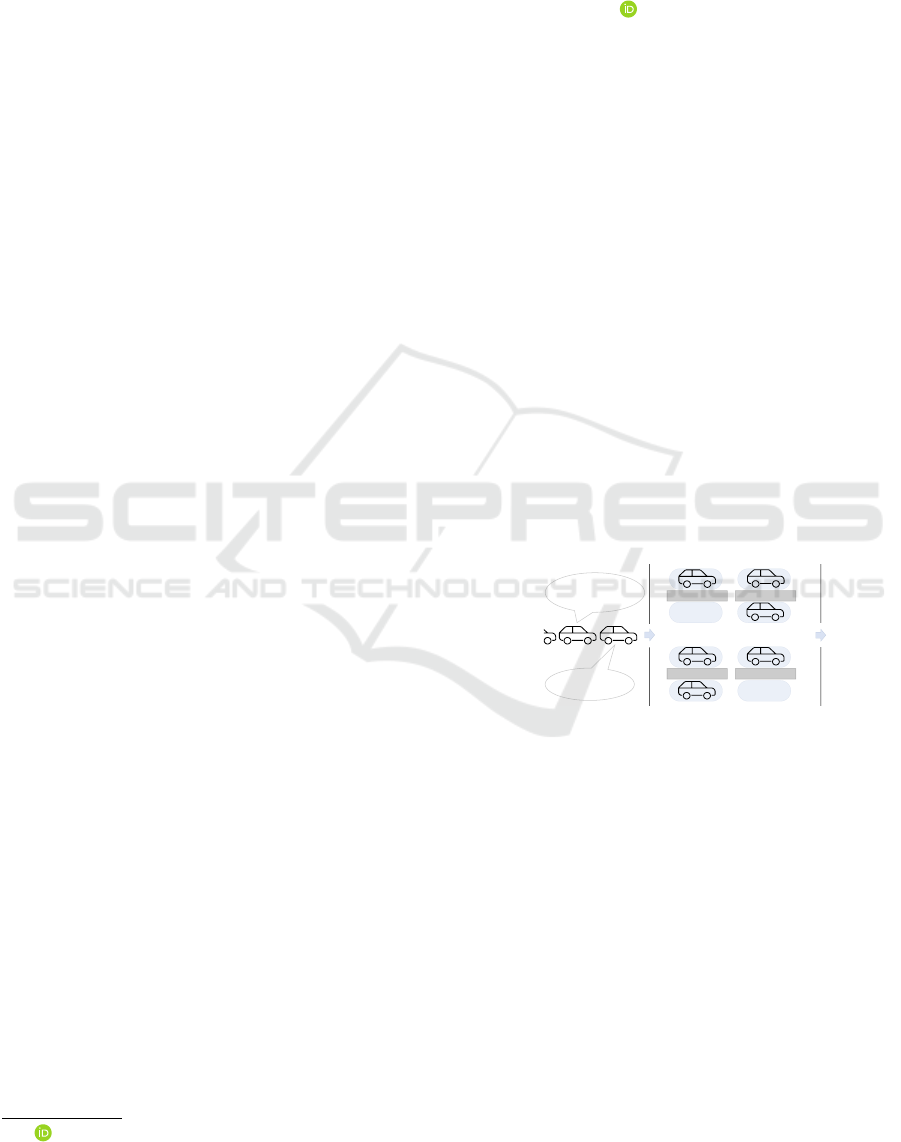
side ones in Japan. This can cause the blocking phe-

nomenon even when some servers in the system are

available like Figure 1. The disadvantages of this phe-

nomenon have been studied using a queueing model

elange et al., 2011).

Type

Mismatch

Blocked by

front vehicle

Machine

Figure 1: Queueing phenomenon that often occurs in GS.

On the other hand, refueling machines with long

hoses can provide service regardless of the position of

the fuel door. Theoretically, the aforementioned phe-

nomenon cannot happen at GSs that install this type

of machine, so this type of machine is preferred in

terms of operational efﬁciency. However, it is difﬁ-

cult to replace all machines due to various constraints

such as costs or safety.

From these backgrounds, our research focuses

on analyzing the queueing system with multi-type

servers and multi-type customers like GSs. In this

research, we consider three types of GSs. In the ﬁrst

type, all machines have a regular hose (dedicated use).

In the second type, all machines have a long hose

(shared use). Finally, a third type is a hybrid form

of the above two types. Then, we model them as

queueing systems and analyze the difference of per-

Machida, Y. and Phung-Duc, T.

A Queueing Analysis of Multi-type Servers and Multi-type Customers System based on Gas Stations.

DOI: 10.5220/0010816100003117

In Proceedings of the 11th International Conference on Operations Research and Enterprise Systems (ICORES 2022), pages 145-152

ISBN: 978-989-758-548-7; ISSN: 2184-4372

145

formances between each type of system.

The structure of this paper is organized as follows.

In Section 2, we explain the queueing models for

three types of GS systems. In Section 3, we present an

analysis of the proposed models in detail. In Section

4, we derive the stability conditions for some systems.

In Section 5, we introduce some performance mea-

sures. In Section 6, we show several numerical exam-

ples. Finally, in Section 7, we conclude this paper and

discuss future works.

2 QUEUEING MODELS

In this section, we model three types of GS systems

as queueing models. A GS may provide various ser-

vices, but here we assume that a GS provides only

refueling service. There are two types of servers in a

GS: dedicated server (regular hose) and shared server

(long hose). In this paper, we consider three types of

systems, i.e., All-Shared servers (AS), All-Dedicated

servers (AD), and Shared-and-Dedicated Mix (SDM).

In all models, customers whose cars are equipped

with a fuel door on the left side (type-L customer)

and right side (type-R customer) arrive at the system

according to Poisson processes with rates λ

and λ

Moreover, service times follow the exponential distri-

bution with a mean of 1/µ. After the service, the lane

becomes empty. In order to analyze models, we set

necessary assumptions. First, we assume that the ar-

rival intervals of customers and the service times of

each server are independent of each other. Second,

the order of services is assumed to be FCFS.

2.1 All-Shared Servers System (AS)

First of all, we describe a queueing model of a GS

that adopts an AS system. AS means that all servers

in the system can provide service for all customers,

so all customers are indiscriminate in this type of sys-

tem. There is no need to distinguish between different

types of customers in this system, so the arrivals of ar-

bitrary customers (type-L or type-R) follow a Poisson

process with rate λ (= λ

+λ

). The schematic of the

model is shown in Figure 2.

If the number of servers is c, a GS that adopts

the AS system can be modeled as an M/M/c queue-

ing system.

𝜆

(𝜆

𝐿

+ 𝜆

𝑅

)

・

𝜇

𝑐

𝜇

Figure 2: The queueing model of AS system GS.

2.2 All-Dedicated Servers System (AD)

Next, we describe a queueing model of a GS that

adopts an AD system. In the AD system, all servers

are either for type-L customers or for type-R cus-

tomers. Thus, this system has two types depending

on how customers line up, queue-divided type and

queue-combined type.

2.2.1 Queue-divided AD System (AD-D)

In this system, customers search for the server that

matches the position of the fuel door on their car and

start getting service. In the AD-D type, if no server is

available, customers line up separately for each type

of their fuel door side. It means that there are two ad-

jacent independent systems. One contains all servers

serving type-L customers, and the other contains all

servers serving type-R customers and each system be-

haves like an AS system.

If the numbers of servers in each system are c

and

+ c

= c), a GS that adopts the AD-D system

can be modeled as two separate M/M/c

and M/M/c

queueing systems.

2.2.2 Queue-combined AD System (AD-C)

Then what if all customers line up together in one

queue? In this type of system, we can observe two

curious phenomena. First, in this type of system, with

customers in the queue, the server that does not match

the customer in the queue head may remain empty and

unused even if the customer behind the head matches

it. Second, from the situation mentioned above, when

the server that matches the customer at the head of

the queue becomes empty, customers behind the head

of the queue might enter the servers simultaneously.

In other words, more than two customers might enter

the servers simultaneously in this type of system. In

this type of system, customers arrive at the system ac-

cording to a Poisson process with rate λ (= λ

+ λ

and the probabilities that a type-L or type-R cus-

tomer is at the head of the queue are λ

(= λ

/λ)

and λ

(= λ

/λ), respectively. The schematic of this

model is shown in Figure 3.

ICORES 2022 - 11th International Conference on Operations Research and Enterprise Systems

146

・

𝜇

𝑐

𝑅

・

𝜇

𝑐

𝐿

𝜆

Type-L

Head

type?

Type-R

L or R

𝜇

Figure 3: The queueing model of AD-C system GS.

In order to analyze this model, we provide the

necessary settings. The numbers of type-L, type-R

servers are c

, c

+ c

= c). We deﬁne N

N ∪{0}, S

:= {0,1,...,c

}, S

:= {0,1,...,c

} (c

= c), S

:= {0,1}, S

∗

:= S

× S

× N

. Let

(t) and C

(t) respectively denote the numbers of

cars staying in type-L and type-R servers in the sys-

tem at time t, where C

(t) ∈ S

, C

(t) ∈ S

. The

type of the fuel door of the customer at the head

of the queue at time t is H(t) ∈ S

. Denote by

L(t) the number of customers in the queue at time

t, where L(t) ∈ N

. After all, we deﬁne X

(t) :=

(L(t), C

(t), C

(t), H(t)). Since S

∗

includes states

that X

(t) cannot reach, we deﬁne S

as the subset of

∗

that excludes unreachable states. In this way, we

can see {X

(t); t ≥ 0} is an irreducible Markov chain

on the state space S

. Based on the above settings, we

analyze this model in Section 3.

2.3 Shared-and-Dedicated-Mix System

(SDM)

Finally, we describe a queueing model of a GS that

adopts the SDM system. SDM means that some

servers in the system are shared, and the others are

dedicated. There is a study on the system of this

mechanism modeled as a loss system for the type that

uses a dedicated server ﬁrst (D-ﬁrst) (Kawashima,

1985). We consider two types of this system about

priority disciplines for server usage: D-ﬁrst and

shared server ﬁrst (S-ﬁrst).

In order to analyze these models, we provide the

necessary settings. The numbers of type-L, type-

R, shared servers are c

, c

+ c

= c).

We deﬁne N

:= N ∪ {0}, S

:= {0, 1, ..., c

}, S

{0,1,...,c

}, S

:= {0, 1, ..., c

} (c

+ c

c), S

:= {0,1}, S

∗

:= S

× S

× N

. Let

(t), C

(t) and C

(t) respectively denote the num-

bers of cars staying in type-L, type-R and shared

servers in the system at time t, where C

(t) ∈

, C

(t) ∈ S

, C

(t) ∈ S

. The type of the fuel door

of the customer at the head of the queue at time t is

H(t) ∈ S

. Denote by L(t) the number of customers

in the queue at time t, where L(t) ∈ N

. After all,

we deﬁne X

(t) := (L(t), C

(t), C

(t), H(t)).

Since S

∗

includes states that X

(t) cannot reach, we

deﬁne S

as the subset of S

∗

that excludes unreach-

able states. In this way, we can see {X

(t); t ≥ 0}

is an irreducible Markov chain on the state space S

Based on the above settings, we analyze this model in

later sections. The difference between the two types

of this system is mentioned in in Section 3.

・

𝜇

𝑐

𝑅

・

𝜇

𝑐

𝐿

𝜆

Type-L

Head

type?

Type-R

L or R

S-first

・

𝜇

𝑐

𝑆

D-first

S-first

𝜇

Priority

law?

Priority

law?

Figure 4: The queueing model of SDM system GS.

3 QUEUEING ANALYSIS

In this section, we deﬁne the inﬁnitesimal generators

for the two models mentioned above: the AD-C sys-

tem and the SDM system, and describe the analysis

of these models. For the other models, the solution

method already exists so that we will derive the per-

formance measures in the later section.

3.1 AD-C System

We construct the transition matrix by separating the

change in the number of customers in the queue.

Then, we represent the inﬁnitesimal generator Q

(1), where O is a zero matrix of appropriate size.







··· L

l+1

···

O O · ·· O O · · ·

O · ·· O O · · ·

··· O O ···

l−1

l−2

··· A

···

l+1

O A

l+1

l−1

··· A

···







(1)

In Q

, l represents the number of type-L and type-

R servers, whichever is greater, plus one. L

(k ≥

1) are the sets given as follows.

:={(0,0,0)} ∪ {(0, 0,1)} ∪ ... ∪ {(0, 0, c

)} ∪{(0, 1, 0)}

∪ ...∪ {(0,c

)}.

:={(k, 0, 0, 0)}∪ {(k, 0, 0,1)} ∪ {(k, 0, 1,0)} ∪ ... ∪{(k,0,c

,1)}

∪ {(k,1,0,0)} ∪ ...∪ {(k,c

,1)}.

A Queueing Analysis of Multi-type Servers and Multi-type Customers System based on Gas Stations

147

In L

, k corresponds to the number of customers

in the queue. Therefore, the block matrices B

and

represent the state transition when the number of

customers in the queue does not change. The block

matrices C

and A

represent the state transition when

the number of customers in the queue increases by

one. A

(2 ≤ k ≤ l + 1) represents the state transition

when the number of customers in the queue decreases

by k − 1. Finally, the block matrix B

(1 ≤ k ≤ l) rep-

resents the state transition when the number of cus-

tomers in the queue decreases from k to zero. For the

elements of each matrix, please refer to the Appendix.

Next, we compute the stationary distribution of

(1). Because {X

(t) ∈ S

; t ≥ 0} deﬁned in the pre-

vious section is a continuous-time Markov chain of

GI/M/1-type, we calculate the stationary distribution

by referring to the method shown in (Adan et al.,

2017). We deﬁne the stationary distribution π

i, j,k,l

(t) for (i, j, k,l) ∈ S

as follows.

i, j,k,l

= lim

t→∞

P(L(t) = i, C

(t) = j, C

(t) = k, H(t) = l),

0, j,k

= lim

t→∞

P(L(t) = 0, C

(t) = j, C

(t) = k).

3.2 SDM System

We consider two priorities in this type of system: D-

ﬁrst and S-ﬁrst, but these only make a difference in

. The differences in B

in consideration of the tran-

sition matrix. The differences are explained in the Ap-

pendix. Finally, we represent the inﬁnitesimal genera-

tor Q

in (2), where O is a zero matrix of appropriate

size.







··· L

l+1

···

O O · ·· O O ·· ·

O · ·· O O ·· ·

··· O O · ··

l−1

l−2

··· A

···

l+1

O A

l+1

l−1

··· A

···







(2)

In Q

, l represents the same meaning as in Q

, L

(k ≥ 1) are the sets given as follows.

:={(0,0,0, 0)} ∪ {(0,0,0,1)} ∪ ... ∪ {(0,0,0,c

)} ∪{(0, 0, 1, 0)}

∪ ...∪ {(0,0,c

)} ∪{(0, 1, 0, 0)}∪ ... ∪{(0, c

)}.

:={(k, 0, 0, 0,0)} ∪ {(k, 0,0,0,1)} ∪{(k,0,0,1, 0)}

∪ ...∪ {(k,0, 0, c

,1)} ∪ {(k,0,1, 0, 0)} ∪ ... ∪ {(k, c

,1)}.

What each block of the transition matrix repre-

sents is the same as in the case of Q

. Please refer

to the Appendix for details.

Next, we compute the stationary distribution of

(2). Because {X

(t) ∈ S

; t ≥ 0} deﬁned in the

previous section is a continuous-time Markov chain

of GI/M/1-type, we calculate the stationary distribu-

tion by referring to the method shown in (Adan et al.,

2017). We deﬁne the stationary distribution π

i, j,k,l,m

of X

(t) for (i, j, k,l, m) ∈ S

as follows.

i, j,k,l,m

= lim

t→∞

P(L(t) = i, C

(t) = j, C

(t) = k, C

(t) = l, H(t) = m),

0, j,k,l

= lim

t→∞

P(L(t) = 0, C

(t) = j, C

(t) = k, C

(t) = l).

4 PERFORMANCE MEASURES

This paper mainly uses the average number of cus-

tomers for each system as a performance measure.

A simple solution has already been shown for

M/M/c type queueing systems. The average numbers

of customers in the AS and AD-D systems are derived

based on (Adan et al., 2017).

The average number of customers in the AD-C

system E

(L) can be derived as follows.

(L) =

∑

j=0

∑

k=0

( j + k)π

0, j,k

∞

∑

i=0

∑

j=0

∑

k=0

∑

l=0

(i + j + k)π

i, j,k,l

The average number of customers in the SDM sys-

tem E

(L) can be derived as follows.

(L) =

∑

j=0

∑

k=0

∑

l=0

( j + k + l)π

0, j,k,l

∞

∑

i=0

∑

j=0

∑

k=0

∑

l=0

∑

m=0

(i + j + k + l)π

i, j,k,l,m

5 NUMERICAL RESULTS

In this section, we present some numerical results

based on the analysis of previous sections. Then, for

all models except AS and AD-D systems, we perform

Monte Carlo simulations to ensure the accuracy of the

numerical results.

5.1 AS, AD-D and AD-C Systems

First of all, we present differences between AS, AD-

D, and AD-C systems. We calculate the average num-

ber of customers in these systems by varying the ar-

rival rate λ and the arrival ratio of type-L to type-R.

The service rate µ is ﬁxed at 40, the number of servers

c is ﬁxed at 8, and the numbers of L and R servers are

the same. The result is shown in Figure 5.

There are some points of interest in this result.

First, in the same arrival rate of the type-L and

type-R, the AS system has the highest performance,

followed by the AD-D system, and the AD-C system

has a considerable performance difference from the

two systems mentioned above. The performance dif-

ference is caused by the blocking phenomenon in the

AD-D system when there are available servers, which

ICORES 2022 - 11th International Conference on Operations Research and Enterprise Systems

148

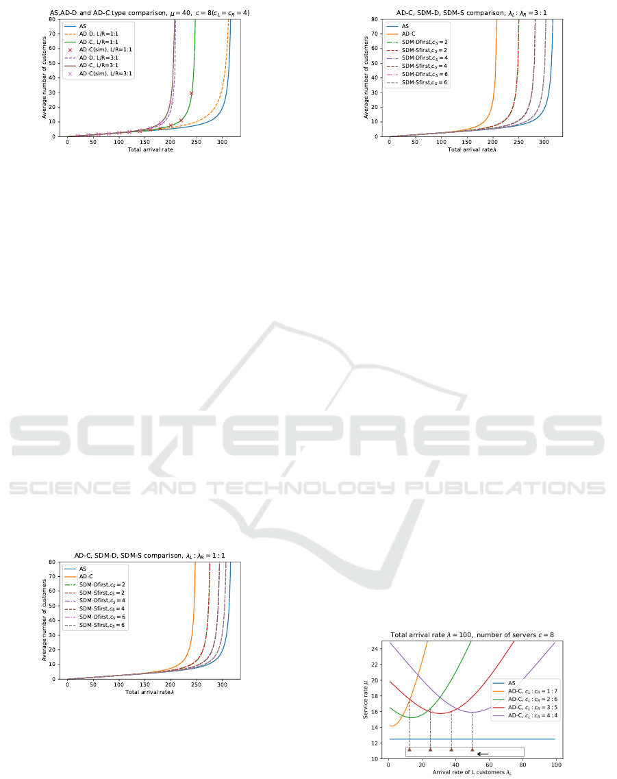
Figure 5: Comparison of AS, AD-D, AD-C systems.

does not occur in the AS system. In the AD-C system,

which has a single standby queue, the phenomenon is

observed more frequently, further degrading the per-

formance of the system.

Second, if there is a signiﬁcant bias in the ar-

rival ratio of type-L to type-R, the performance dif-

ference between AD-D and AD-C becomes smaller.

The more signiﬁcant bias in the arrival ratio of type-L

to type-R, the more the two systems will approximate

a system where only one type of server is used on each

side.

5.2 AD-C and SDM Systems

Next, we present differences between AD-C and two

types of SDM systems. We are interested in the effect

of the number of shared servers c

in two types of

SDM systems. We calculate these systems by varying

λ and c

. The service rate µ and the number of servers

in the system c are the same as the comparison in Sec-

tion 5.1. The results are shown in Figure 6 and Figure

Figure 6: Comparison of AD-C system and SDM systems

without bias of arrival rate.

We observe two interesting points in the results.

First, according to Figure 5, Figure 6 and Figure 7,

the performance of the SDM system is in the middle

between the AD-C system and the AS system, and

each additional shared server leads to an ever-smaller

improvement of the performance of the SDM system.

Second, in the two types of SDM systems, there is not

much difference in performance between SDM-Dﬁrst

Figure 7: Comparison of AD-C system and SDM systems

with the large bias of arrival rate.

and SDM-Sﬁrst, and in situations where the system

is approaching instability, there is little difference be-

tween the two types of systems. Furthermore, there is

little difference between the two types of SDM sys-

tems, whether the shared server with higher utility is

used ﬁrst or the dedicated server is used ﬁrst in situ-

ations with no customer in the queue. Since the two

types of systems are considered precisely the same

when there is a queue of customers, our model, which

allows for an inﬁnite buffer, does not show a signif-

icant difference, especially when the number of cus-

tomers in the queue is likely to increase. If this system

is changed to the loss system with no customer in the

queue or has a much larger number of servers, the dif-

ferences between the two types of systems are likely

to arise clearly.

5.3 Comparison in Stability Conditions

of AD-C System

At last, we present a comparison of the stability con-

ditions of the AD-C system varying the L-R ratio of

the number of servers. We calculate the stability con-

ditions of the AD-C system. In the experiment, we

set λ = 100, c = 8 and let the arrival rate of type-L

customers vary. The results are shown in Figure 8.

1:7

L-R arrival ratio

2:6

3:5

4:4

Figure 8: Comparison of L-R server ratio about AD-C sys-

tem.

There are two notable points in the results.

First, the greater the bias of the L-R ratio of the

number of servers, the smaller the minimum service

A Queueing Analysis of Multi-type Servers and Multi-type Customers System based on Gas Stations

149

rate required for system stability. In other words, the

more biased the L-R ratio of the number of servers is,

the system can be operated with less service capacity

when the arrival left-right ratio is optimal. This occurs

for the same reason as in the previous result: the more

signiﬁcant bias the L-R server ratio and arrival ratio

of type-L to type-R are, the more the system behaves

like a smaller AS system, hence this result.

Second, intuitively, it seems to be most efﬁcient

for the system when the L-R ratio of the number of

servers and arrival ratio of type-L to type-R is the

same. However, the result is often not so. In Figure

8, the lower markers represent the values at which the

arrival ratios of type-L to type-R are the same as each

server L-R ratio. The greater the bias in the server L-R

ratio, the greater the difference between the most ef-

ﬁcient arrival ratio of type-L to type-R and the server

L-R ratio. It is thought to be caused for the risk of

the minor-type customers at the head of the queue.

The larger the bias in the server L-R ratio, the more

likely it is that when a minor-type customer lines up

at the head of the queue, many major-type customers

will line up behind. In order to avoid this waste, it is

thought to be desirable that the arrival ratio of type-L

to type-R is larger bias than the server L-R ratio, and

in such a situation, major-type customers are more

likely to be at the head of the queue, making it dif-

ﬁcult for the aforementioned risk to occur.

6 CONCLUSION

We have modeled the systems with multi-type servers

and multi-type customers based on gas stations by

queueing systems. In this paper, we have evaluated

some differences among the systems. First, we com-

pared an AS system and the two types of AD sys-

tems. Second, we observed the impact of the number

of shared servers in the two types of SDM systems.

Third, we considered the effect of servers and arrival

left-right ratio in the AD-C system.

Finally, we consider the future works. In this

study, we have modeled the systems of gas stations

in simpliﬁed situations. However, in reality, the gas

station systems have much more complexity, so one

may consider incorporating more complex and real-

istic situations. First, for example, some customers

can get service from all types of servers, like motor-

cycles. Second, in the point of view about queue cre-

ation, there exists a system that is neither AD-D nor

AD-C, where customers are divided by their type in

the middle of the queue. Studies of similar systems

exist (M

elange et al., 2020), but there is no mention of

multiple servers’ cases. Second, due to the small size

of the gas station site, there are incidents where cus-

tomers cannot leave after the service and customers in

the queue cannot enter the available servers. This phe-

nomenon has already been studied earlier (Teimoury

et al., 2011; Jiang, 2018), but their models are single-

row services, which are more straightforward than the

actual GS multi-row service. In addition, there are

various kinds of factors that seem to affect a gas sta-

tion system. For example, customers also enter the

system for other services such as car washing, then

join the queue for fueling afterward. In this case,

the new system may be modeled as a tandem queue

where multiple types of services are available, and

more variables need to be added to capture such com-

plexity.

ACKNOWLEDGEMENTS

The research of the second author is supported in part

by JSPS KAKENHI Grant Number 21K11765.

REFERENCES

Adan, I., van Leeuwaarden, J., and Selen, J. (2017). Anal-

ysis of structured markov processes. arXiv preprint

arXiv:1709.09060.

Jiang, T. (2018). Analysis of a tollbooth tandem queue

with two-class customers and two heterogeneous ded-

icated servers. Asia-Paciﬁc Journal of Operational

Research, 35(06):1850043.

Kawashima, K. (1985). An approximation of a loss sys-

tem with two heterogeneous types of calls. Journal of

the Operations Research Society of Japan, 28(2):163–

177.

elange, W., Bruneel, H., Steyaert, B., and Walraevens,

J. (2011). A two-class continuous-time queueing

model with dedicated servers and global fcfs service

discipline. In International Conference on Analyti-

cal and Stochastic Modeling Techniques and Applica-

tions, pages 14–27. Springer.

elange, W., Walraevens, J., and Bruneel, H. (2020).

Performance analysis of a continuous-time two-class

global ﬁrst-come-ﬁrst-served queue with two servers

and presorting. Annals of Operations Research.

Ministry of Land, Infrastructure, Transport and Tourism,

Japan (2021). Statistics on the number of vehi-

cles owned. https://www.mlit.go.jp/statistics/details/

jidosha list.html. Accessed : 2021-09-05.

Next Generation Vehicle Promotion Center, Japan (2020).

Statistics on the number of evs and like vehicles

owned. http://www.cev-pc.or.jp/tokei/hanbai.html.

Accessed : 2021-09-05.

Teimoury, E., Yazdi, M. M., Haddadi, M., and Fathi,

M. (2011). Modelling and improvement of non-

standard queuing systems: a gas station case study.

ICORES 2022 - 11th International Conference on Operations Research and Enterprise Systems

150

International Journal of Applied Decision Sciences,

4(4):324–340.

APPENDIX

We describe each of the block matrices used in the

inﬁnitesimal generators deﬁned in Section 3. In the

following, the element in the i−th row from the top

and j−th column from the left of a block matrix is

called the (i, j) element. For instance, the (i, j) ele-

ment of a block matrix A is denoted as A

i, j

. Note that

the matrix components of the undeﬁned part in each

block matrix are all zero.

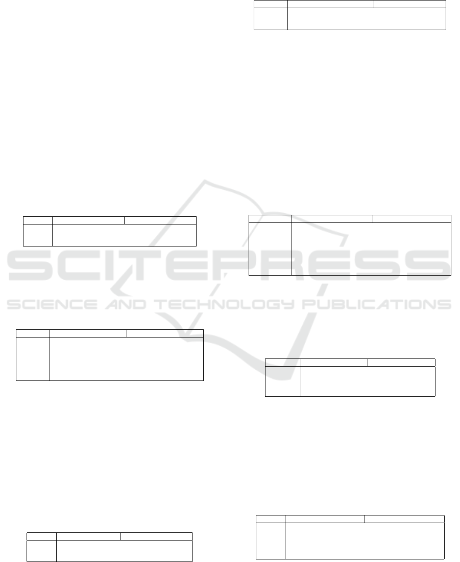
First, we describe each of the block matrices used

in the inﬁnitesimal generator about the AD-C system.

is a ((c

+ 1) × (c

+ 1) × 2)-order square ma-

trix that represents the transition of the number of cus-

tomers in the queue from i to i + 1 (i ≥ 1). Thus, each

element (A

)

i, j

is deﬁned as follows.

Table 1: Matrix components of A

)

i, j

i j

λ (m + 1) × (c

+ 1) × 2 (m + 1) × (c

+ 1) × 2

λ (c

+ 1) + n) × 2 +1 (c

+ 1) + n) × 2 +1

if (0 ≤ m ≤ c

, 0 ≤ n ≤ c

)

is a ((c

+ 1) × (c

+ 1))-order square matrix

that represents the transition of states when the num-

ber of customers in the queue is zero. Each element

)

i, j

is deﬁned as follows.

Table 2: Matrix components of B

)

i, j

i j

+ 1) × m + n + 1 (c

+ 1) × (m + 1) +n + 1

(m + 1)µ (c

+ 1) × (m + 1) +n + 1 (c

+ 1) × m + n + 1

if (0 ≤ m ≤ c

− 1, 0 ≤ n ≤ c

)

+ 1) × m + n + 1 (c

+ 1) × m + n + 2

(n + 1)µ (c

+ 1) × m + n + 2 (c

+ 1) × m + n + 1

if (0 ≤ m ≤ c

, 0 ≤ n ≤ c

)

Denoting I := {1,2,...,(c

+ 1) × (c

+ 1)}, J :=

{1,2,...,(c

+ 1)× (c

+ 1)× 2}, i ∈ I, we deﬁne the

diagonal components of B

as follows.

)

i,i

= −

∑

j∈I\{i}

)

i, j

∑

j∈J

)

i, j

is a matrix of size ((c

+1)×(c

+1))×((c

1) × (c

+ 1) × 2) that represents the transition of the

number of customers in the queue from zero to 1.

Each element (C

)

i, j

is deﬁned as follows.

Table 3: Matrix components of C

)

i, j

i j

× (c

+ 1) + n + 1 (c

+ 1) + n) × 2 + 1

(m + 1) × (c

+ 1) (m + 1) × (c

+ 1) × 2

if ( 0 ≤ m ≤ c

, 0 ≤ n ≤ c

)

is a ((c

+ 1) × (c

+ 1) × 2)-order square ma-

trix that represents the transition of states when the

number of customers in the queue is greater than or

equal to 1. Each element(A

)

i, j

is deﬁned as follows.

Table 4: Matrix components of A

)

i, j

i j

(m + 1)µ (m + 2) × (c

+ 1) × 2 (m + 1) × (c

+ 1) × 2

(n + 1)µ (c

+ 1) + (n + 1)) ×2 + 1 (c

+ 1) + n) × 2 + 1

if ( 0 ≤ m ≤ c

− 1, 0 ≤ n ≤ c

− 1)

We deﬁne the diagonal components of A

when

the number of customers in the queue is l as follows.

)

i,i

= −

∑

j∈I

)

i, j

∑

k=2

∑

j∈J

)

i, j

∑

j∈I\{i}

)

i, j

∑

j∈J

)

i, j

(k ≥ 2) is a ((c

+ 1) × (c

+ 1) × 2)-order

square matrix that represents the transition that the

number of customers in the queue decreases by k − 1

but not to zero. Note that the probability that a cus-

tomer in the queue is type-L is λ

/λ (:= λ

) and the

probability that a customer in the queue is type-R is

/λ (:= λ

). Each element (A

)

i, j

is deﬁned as fol-

lows.

Table 5: Matrix components of A

)

i, j

i j

µλ

0k−2

+ 1) + (n + 1))

×2 − 1

+ 1) + (k + n − 1))

×2 − 1

µλ

0k−1

((c

+ 1)(c

+ 1) + (2 − k))

×2 − 1

+ 1) × (c

+ 1) × 2

µλ

0k−2

(m + 1) × (c

+ 1) × 2 (k +m − 1)× (c

+ 1) × 2

µλ

0k−1

− k + 3) × (c

+ 1) × 2 (c

+ 1) × (c

+ 1) × 2 − 1

if ( 0 ≤ m ≤ c

+ 2 − k, 0 ≤ n ≤ c

+ 2 − k)

(k ≥ 1) is a matrix of size ((c

+1)×(c

+1)×

2)×((c

+1)×(c

+1)) that represents the transition

of the number of customers in the queue from k to

zero. Each element (B

)

i, j

is deﬁned as follows.

Table 6: Matrix components of B

)

i, j

i j

µλ

0k−1

+ 1) + (n + 1))

×2 − 1

+ 1) + n + k − 1

µλ

0k−1

(m + 1) × (c

+ 1) × 2 (m + k)(c

+ 1)

if ( 0 ≤ m ≤ c

+ 1 − k, 0 ≤ n ≤ c

+ 1 − k)

Second, we describe each block matrices used in

the inﬁnitesimal generator about two types of SDM

systems.

is a ((c

+ 1) × (c

+ 1) × 2)-order

square matrix that represents the transition of the

number of customers in the queue from i to i + 1 (i ≥

1). Each element (A

)

i, j

is deﬁned as follows.

Table 7: Matrix components of A

)

i, j

i j

(m + 1) × (c

+ 1)

×(c

+ 1) × 2

(m + 1) × (c

+ 1)

×(c

+ 1) × 2

+ 1) + n) × (c

+ 1)

×2 + 1

+ 1) + n) × (c

+ 1)

×2 + 1

if (0 ≤ m ≤ c

, 0 ≤ n ≤ c

)

is a ((c

+ 1) × (c

+ 1))-order

square matrix that represents the transition of states

A Queueing Analysis of Multi-type Servers and Multi-type Customers System based on Gas Stations

151

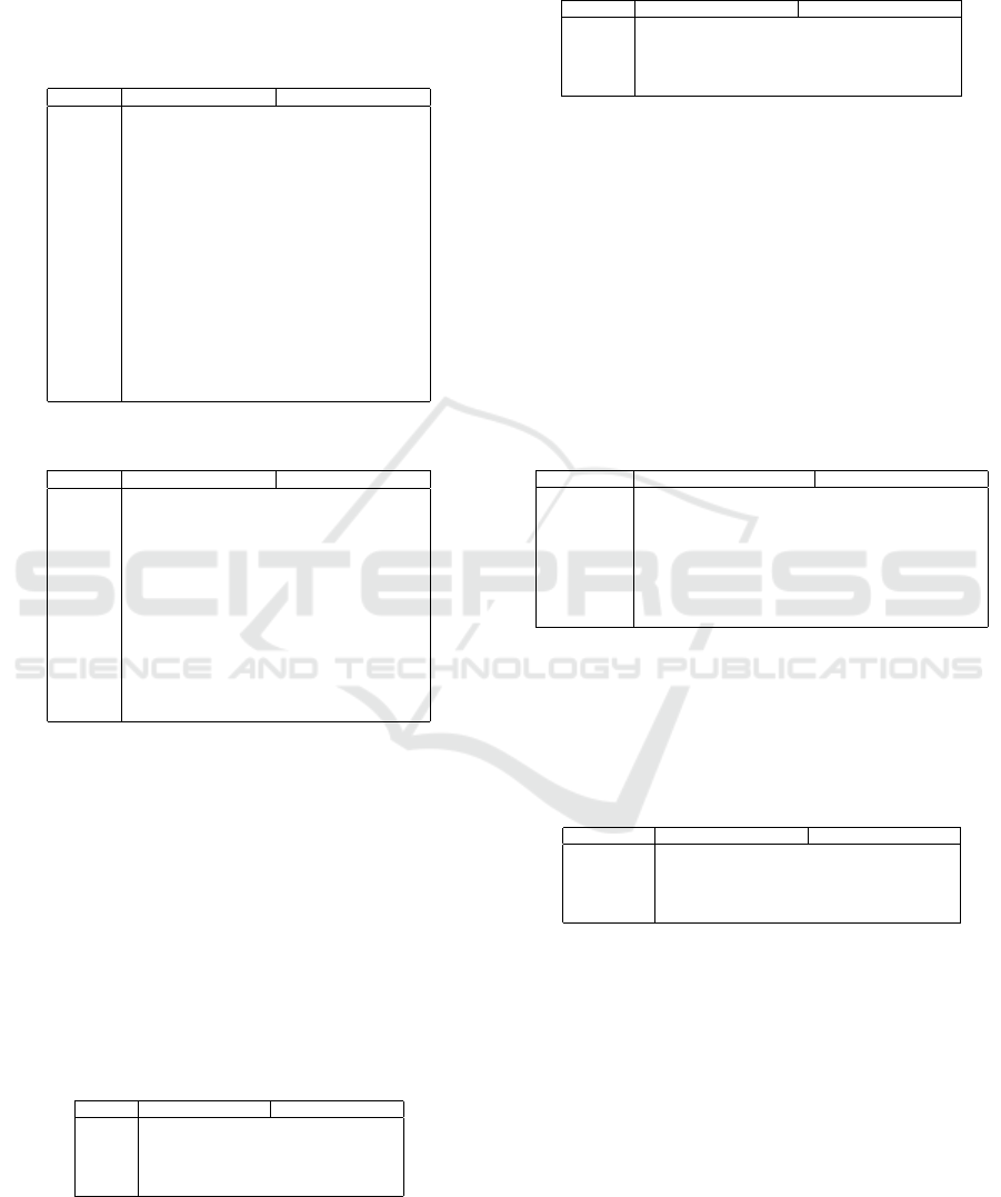
when the number of customers in the queue is zero.

There are two types in the SDM system. The only

difference between the two types is the components

of B

. Each element of B

of D-ﬁrst (B

)

i, j

and S-

ﬁrst (B

)

i, j

are deﬁned as follows.

Table 8: Matrix components of B

)

i, j

i j

(l × (c

+ 1) + m)

×(c

+ 1) + n + 1

((l + 1) ×(c

+ 1) + m)

×(c

+ 1) + n + 1

(l + 1)µ

((l + 1) ×(c

+ 1) + m)

×(c

+ 1) + n + 1

(l × (c

+ 1) + m)

×(c

+ 1) + n + 1

if (0 ≤ m ≤ c

− 1, 0 ≤ n ≤ c

, 0 ≤ n ≤ c

)

(l × (c

+ 1) + m)

×(c

+ 1) + n + 1

(l × (c

+ 1) + m + 1)

×(c

+ 1) + n + 1

(m + 1)µ

(l × (c

+ 1) + m + 1)

×(c

+ 1) + n + 1

(l × (c

+ 1) + m)

×(c

+ 1) + n + 1

if (0 ≤ m ≤ c

, 0 ≤ n ≤ c

− 1, 0 ≤ n ≤ c

)

× (c

+ 1) + m)

×(c

+ 1) + n + 1

× (c

+ 1) + m)

×(c

+ 1) + n + 2

(l × (c

+ 1) + c

)

×(c

+ 1) + n + 1

(l × (c

+ 1) + c

)

×(c

+ 1) + n + 2

× (c

+ 1) + c

)

×(c

+ 1) + n + 1

× (c

+ 1) + c

)

×(c

+ 1) + n + 2

(n + 1)µ

(l × (c

+ 1) + m)

×(c

+ 1) + n + 2

(l × (c

+ 1) + m)

×(c

+ 1) + n + 1

if (0 ≤ m ≤ c

, 0 ≤ n ≤ c

− 1)

Table 9: Matrix components of B

)

i, j

i j

(l × (c

+ 1) + m)

×(c

+ 1) + c

+ 1

((l + 1) ×(c

+ 1) + m)

×(c

+ 1) + c

+ 1

(l + 1)µ

((l + 1) ×(c

+ 1) + m)

×(c

+ 1) + n + 1

(l × (c

+ 1) + m)

×(c

+ 1) + c

+ 1

if (0 ≤ m ≤ c

− 1, 0 ≤ n ≤ c

, 0 ≤ n ≤ c

)

(l × (c

+ 1) + m)

×(c

+ 1) + c

+ 1

(l × (c

+ 1) + m + 1)

×(c

+ 1) + c

+ 1

(m + 1)µ

(l × (c

+ 1) + m + 1)

×(c

+ 1) + c

+ 1

(l × (c

+ 1) + m)

×(c

+ 1) + c

+ 1

if (0 ≤ m ≤ c

, 0 ≤ n ≤ c

− 1, 0 ≤ n ≤ c

)

(l × (c

+ 1) + m)

×(c

+ 1) + n + 1

(l × (c

+ 1) + m)

×(c

+ 1) + n + 2

(n + 1)µ

(l × (c

+ 1) + m)

×(c

+ 1) + n + 2

(l × (c

+ 1) + m)

times(c

+ 1) + n + 1

if (0 ≤ m ≤ c

, 0 ≤ n ≤ c

− 1)

Denoting I := {1,2,...,(c

+1) × (c

1)}, J := {1, 2, ..., (c

+ 1) × (c

+ 1) ×

2}, i ∈ I, we deﬁne the diagonal components of

, B

as follows.

D(S)

)

i,i

= −

∑

j∈I\{i}

D(S)

)

i, j

∑

j∈J

)

i, j

is a matrix of size ((c

+ 1) × (c

1)) × ((c

+ 1) × (c

+ 1) × 2) that repre-

sents the transition of the number of customers in the

queue from zero to 1. Each element (C

)

i, j

is deﬁned

as follows.

Table 10: Matrix components of C

)

i, j

i j

× (c

+ 1) + m)

×(c

+ 1) + 1

× (c

+ 1) + m)

×2 + 1

(l + 1) ×(c

+ 1)

×(c

+ 1)

(l + 1) ×(c

+ 1)

×(c

+ 1) × 2

if(0 ≤ l ≤ c

, 0 ≤ m ≤ c

)

is a ((c

+ 1) × (c

+ 1) × 2)-order

square matrix that represents the transition of states

when the number of customers in the queue is greater

than or equal to 1. Each element (A

)

i, j

is deﬁned as

follows.

Table 11: Matrix components of A

)

i, j

i j

(l + 1)µ

(l + 2) ×(c

+ 1)

×(c

+ 1) × 2

(l + 1) ×(c

+ 1)

×(c

+ 1) × 2

(m + 1)µ

× (c

+ 1) + (m + 2))

×(c

+ 1) × 2 − 1

× (c

+ 1) + (m + 1))

×(c

+ 1) × 2 − 1

if(0 ≤ l ≤ c

− 1, 0 ≤ m ≤ c

− 1)

We deﬁne the diagonal components of A

when

the number of customers in the queue is l as follows.

)

i,i

= −

∑

j∈I

)

i, j

∑

k=2

∑

j∈J

)

i, j

∑

j∈I\{i}

)

i, j

∑

j∈J

)

i, j

(k ≥ 2) is a ((c

+1)× (c

+1)× 2)-

order square matrix that represents the transition of

the number of customers in the queue decreasing by

k − 1 but not to zero. We deﬁne c

and c

as the

sum of the type-L servers and shared servers, type-

R servers and shared servers. Each element(A

)

i, j

deﬁned as follows.

Table 12: Matrix components of A

)

i, j

i j

µλ

0k−2

× (c

+ 1) + m + 1)

×(c

+ 1) × 2 − 1

× (c

+ 1) + k + m − 1)

×(c

+ 1) × 2 − 1

µλ

0k−1

((c

+ 1) × (c

+ 1) + 2 − k)

×(c

+ 1) × 2 − 1

+ 1) × (c

+ 1)

×(c

+ 1) × 2

µλ

0k−2

(l + 1) ×(c

+ 1)

×(c

+ 1) × 2

(k + l − 1) × (c

+ 1)

×(c

+ 1) × 2

µλ

0k−−1

+ 3 − k) × (c

+ 1)

×(c

+ 1) × 2

+ 1) × (c

+ 1)

×(c

+ 1) × 2 − 1

if(0 ≤ l ≤ c

+ 2 − k, 0 ≤ m ≤ c

+ 2 − k)

(k ≥ 1) is a matrix of size ((c

+1)×(c

+1)×

+ 1) × 2) × ((c

+ 1) × (c

+ 1)) that

represents the transition of the number of customers

in the queue from k to zero. Each element(B

)

i, j

deﬁned as follows.

Table 13: Matrix components of B

)

i, j

i j

µλ

0k−1

× (c

+ 1) + m + 1)

×(c

+ 1) × 2 − 1

× (c

+ 1) + k + m)

×(c

+ 1)

µλ

0k−−1

(l + 1) ×(c

+ 1)

×(c

+ 1) × 2

(k + l) × (c

+ 1)

×(c

+ 1)

if(0 ≤ l ≤ c

+ 1 − k, 0 ≤ m ≤ c

+ 1 − k)

ICORES 2022 - 11th International Conference on Operations Research and Enterprise Systems

152