Method for Improving Quality of Adversarial Examples

Duc-Anh Nguyen

1 a

, Kha Do Minh

1 b

, Duc-Anh Pham

2 c

and Pham Ngoc Hung

1 d

VNU University of Engineering and Technology (VNU-UET),

Building E3, 144 Xuan Thuy Road, Cau Giay District, Hanoi, Vietnam

University of Transport Technology, 54 Trieu Khuc Road, Thanh Xuan District, Hanoi, Vietnam

Keywords:

Adversarial Example Generation, Deep Neural Network, Robustness, Autoencoder.

Abstract:

To evaluate the robustness of DNNs, most of the adversarial methods such as FGSM, box-constrained L-

BFGS, and ATN generate adversarial examples with small L

-norm. However, these adversarial examples

might contain many redundant perturbations. Removing these perturbations increases the quality of adver-

sarial examples. Therefore, this paper proposes a method to improve the quality of adversarial examples by

recognizing and then removing such perturbations. The proposed method includes two phases namely the au-

toencoder training phase and the improvement phase. In the autoencoder training phase, the proposed method

trains an autoencoder that learns how to recognize redundant perturbations. In the second phase, the pro-

posed method uses the trained autoencoder in combination with the greedy improvement step to produce more

high-quality adversarial examples. The experiments on MNIST and CIFAR-10 have shown that the proposed

method could improve the quality of adversarial examples signiﬁcantly. In terms of L

-norm, the distance

decreases by about 82%-95%. In terms of L

-norm, the distance drops by around 56%-81%. Additionally,

the proposed method has a low computational cost. This shows the potential ability of the proposed method

in practice.

1 INTRODUCTION

Deep neural networks (DNNs) are widely used in im-

age classiﬁcation (Carlini and Wagner, 2016; Cire-

gan et al., 2012; Sultana et al., 2019). Recent re-

search has shown that even DNNs achieve high ac-

curacy on the training set, these models might suffer

from poor robustness (Baluja and Fischer, 2017; Car-

lini and Wagner, 2016; Eniser et al., 2019; Goodfel-

low et al., 2015; Gopinath et al., 2019; Kurakin et al.,

2016; Zhang et al., 2019). The robustness of DNNs

measures the degree to which these DNNs work cor-

rectly in the presence of slight perturbations. Term

adversarial example is used to call an original input

image added slight perturbations. While the original

input images must be recognized correctly by the at-

tacked DNNs, these DNNs are not able to detect the

label of adversarial examples properly. Due to the ex-

istence of adversarial examples, this poses a security

concern on the robustness of DNNs.

https://orcid.org/0000-0002-6337-6254

https://orcid.org/0000-0002-1917-8314

https://orcid.org/0000-0002-6017-6740

https://orcid.org/0000-0002-5584-5823

Targeted attack is a well-known approach to gen-

erate adversarial examples. These adversarial exam-

ples could be used as evidence to demonstrate the ro-

bustness of DNNs. There are many methods in this

approach such as FGSM (Goodfellow et al., 2015),

BIS (Kurakin et al., 2016), ATN (Baluja and Fischer,

2017), Carnili-Wagner (Carlini and Wagner, 2016),

box-constrained L-BFGS (Szegedy et al., 2014), etc.

The general purpose of these methods is to generate

adversarial examples close to the original input im-

ages and classiﬁed as a target label. The target label

is different from the ground-truth label. To compute

the distance between adversarial examples and origi-

nal input images, the most common metric is L

-norm

metric. Some popular L

-norm could be referred to

-norm (Carlini and Wagner, 2016; Gopinath et al.,

2019), L

-norm (Baluja and Fischer, 2017; Carlini

and Wagner, 2016; Szegedy et al., 2014), and L

∞

norm (Goodfellow et al., 2015; Kurakin et al., 2016).

Although these methods could generate adversar-

ial examples with small L

-norm, these methods are

still confronted by the problem of redundant pertur-

bation. Speciﬁcally, these methods suggest their own

objective functions containing the objective functions

of the attacked DNNs. The objective functions of

214

Nguyen, D., Do Minh, K., Pham, D. and Hung, P.

Method for Improving Quality of Adversarial Examples.

DOI: 10.5220/0010814400003116

In Proceedings of the 14th International Conference on Agents and Artiﬁcial Intelligence (ICAART 2022) - Volume 2, pages 214-225

ISBN: 978-989-758-547-0; ISSN: 2184-433X

these methods are minimized as much as possible.

The result of the minimization is a set of adversar-

ial examples with small L

-norm. However, due to

the non-linear property of DNNs, minimizing their

deﬁned objective functions might struggle at the lo-

cal minimum. It means that the quality of adversarial

examples might not be optimal. In other words, ad-

versarial examples still might contain redundant per-

turbations. A perturbation is redundant if removing

it from an adversarial example does not change the

label of this adversarial example. If such redundant

perturbations are removed from adversarial examples,

the value of their deﬁned objective functions would be

smaller. The L

-norm between the original input im-

ages and adversarial examples could be reduced sig-

niﬁcantly. As the result, this makes the adversarial

examples closer to the original input images.

To mitigate the above problem, this paper pro-

poses a method that detects and removes redundant

perturbations with a low computational cost. We fo-

cus on L

-norm and L

-norm metrics. The proposed

method includes two main phases, namely the autoen-

coder training phase and the improvement phase. In

the autoencoder training phase, the proposed method

trains an autoencoder. The purpose of this autoen-

coder is to recognize redundantly adversarial features

in adversarial examples. An adversarial feature is re-

dundant if it contains redundant perturbation. There-

fore, it should be restored to its original value. The

original value is the value of the corresponding fea-

ture on the original input image. In the improvement

phase, an adversarial example is fed into the trained

autoencoder to generate the ﬁrst version of the im-

proved adversarial example. However, because this

improved adversarial example might still contain re-

dundant perturbations, the proposed method uses a

greedy improvement step to remove these perturba-

tions.

The experiments on the MNIST dataset (Lecun

et al., 1998a) and the CIFAR-10 dataset (Krizhevsky,

2012) have shown that the proposed method could en-

hance the quality of adversarial examples consider-

ably. The proposed method is compared with a greedy

method. As a result, the introduced method could

achieve the L

-norm reduction rate of 82%-95% and

the L

-norm reduction rate of 56%-81%. Addition-

ally, the proposed method could improve the qual-

ity of new adversarial examples with a low compu-

tational cost. It takes several seconds to improve the

quality of about 1,000 adversarial examples.

The rest of this paper is organized as follows. Sec-

tion 2 provides the background of this topic. Section 3

describes a motivating example of this research. Sec-

tion 4 describes a greedy method to enhance the qual-

ity of adversarial examples. The overview of the pro-

posed method is shown in Section 5. Next, Section 6

presents the experiments to demonstrate the advan-

tages of the proposed method. Section 7 delivers the

overview of the related research. Finally, the conclu-

sion is described in Section 8.

2 BACKGROUND

In this section, the paper provides the background

about the adversarial example generation topic. We

ﬁrst review the basic concept of DNNs and the tar-

geted attack. We then describe the overview of the

stacked convolutional autoencoder. Finally, this pa-

per reviews well-known adversarial example genera-

tion methods using L

-norm metric.

2.1 Deep Neural Network

A DNN M is made of h successive layers. A simple

representation of a DNN is as follows:

M(x) = Q

h−1

h−2

(...(Q

(x)))) ∈ R

(1)

where x ∈ R

is an input image of the DNN classi-

ﬁer, d is the number of features, k is the number of

classes, h is the number of layers, and Q

is the i-th

layer. The input layer and the output layer are Q

and Q

h−1

, respectively. Each layer has one activa-

tion function. Some popular activation functions are

ReLU and softmax. The output of the DNN M is a

probability vector of size k. The predicted label of an

input x is computed by argmaxM(x).

2.2 Targeted Attack

The targeted attack is a popular approach to generate

adversarial examples. Given an input image x and a

target label y

∗

, the purpose of the targeted attack is

modifying this input to generate an adversarial exam-

ple x

. This adversarial example is classiﬁed as y

∗

which is different from the ground-truth label of x.

Additionally, x

should be close to x as much as pos-

sible.

Deﬁnition 1 (Adversarial Feature). Given an input

image x and its corresponding adversarial example

x’, a feature x

on x’ is considered as adversarial fea-

ture if and only if x

6= x

, where x

is the original value

of x

Deﬁnition 2 (Redundant Perturbation). Consider an

adversarial feature, its perturbation β is redundant if

and only if x’ and (x’ − β) are labelled the same. In

this case, this feature is called a redundantly adver-

sarial feature.

Method for Improving Quality of Adversarial Examples

215

Deﬁnition 3 (Improved Adversarial Example). An

improved adversarial example x’

is the result of re-

moving redundant perturbations from its correspond-

ing adversarial example x’, in which x’

and x’ are

assigned to the same label by M.

-norm. To measure the distance between origi-

nal input images and adversarial examples, the com-

monly used metric is L

-norm. Given an input image

x, its corresponding adversarial example x

should be

identical to x under L

-norm metric as much as possi-

ble. The main reason is that it does not make sense if

an adversarial example is too different from the orig-

inal input image. The L

-norm distance between the

input image x and its adversarial example x

is for-

mally deﬁned as follows:

(x,x

) =

∑

− x

)

(2)

2.3 Stacked Convolutional Autoencoder

A stacked convolutional autoencoder considers the

structure of 2D and 3D images. This type of autoen-

coder includes one encoder and one decoder. In the

encoder part, a layer can be down-sampling, convo-

lutional, and fully-connected. In the decoder part,

a layer can be up-sampling, deconvolutional, and

fully-connected. The typical objective function of the

stacked convolutional autoencoder is as follows:

∑

out

) (3)

where x

is the input image on the training set, x

out

is the corresponding reconstructed image of x

. The

distance between x

and x

out

is computed by using

metric L

-norm.

2.4 Popular Targeted L

-norm Attack

This part describes three common targeted attacks us-

ing L

-norm metric. While FGSM uses L

∞

-norm,

box-constrained L-BFGS and ATN use L

-norm. To

generate an adversarial example, these methods could

add perturbations to all features on an input image.

2.4.1 Box-constrained L-BFGS

Szegedy et al. (2014) proposed box-constrained L-

BFGS to generate adversarial examples. Their

method solves the following box-constrained opti-

mization problem:

minimize (1 − c) · L

,x) + c · f (y

∗

,M(x

))

such that x

∈ [0, 1]

(4)

where f is a function to compute the difference be-

tween M(x

) and the target label y

∗

, and c is the

weight to balance two terms. A common choice of

f is cross-entropy.

2.4.2 FGSM

Goodfellow et al. (2015) proposed a fast gradient sign

method (FGSM) to generate adversarial examples.

Speciﬁcally, given an input image x, and a value ε,

its corresponding adversarial example x

is computed

as follows:

= x − ε · sign(∇

f (x,y

∗

,ζ)) (5)

where sign(.) returns the sign of ∇

f (x,y

∗

,ζ) and ε

is a positive value to shift values of all features in x.

2.4.3 ATN

Baluja and Fischer (2017) proposed ATN to generate

adversarial examples based on an autoencoder. The

input of the autoencoder is an input image x. The

output is an adversarial example x

. The authors sug-

gested using L

-norm to compute the distance be-

tween x

and x. The objective function of sample x

is as follows:

(1 − φ) · L

(x,x

) + φ · L

(M(x

),r

(M(x),y

∗

)) (6)

where r

(.) is a reranking function, φ is the weight

between the two terms of the objective function,

(M(x

),r

(M(x),y

∗

)) is the L

-norm distance be-

tween M(x

) and the expected probability vector

(M(x),y

∗

The reranking function r

(.) is deﬁned as follows:

(M(x),y

∗

)

= norm



α · max(M(x)) i f i = y

∗

M(x)

otherwise



i∈{0..k−1}



(7)

where α > 1 is used to specify how much larger y

∗

should be than max(M(x)). Function norm(·) nor-

malizes its input to a probability distribution.

3 MOTIVATING EXAMPLE

Many methods are proposed to generate adversar-

ial examples with small L

-norm. For L

-norm,

some well-known methods could be referred to

Carnili-Wagner L

(Carlini and Wagner, 2016) and

DeepCheck (Gopinath et al., 2019). Concerning L

norm, Carnili-Wagner L

(Carlini and Wagner, 2016),

box-constrained L-BFGS (Szegedy et al., 2014), and

ICAART 2022 - 14th International Conference on Agents and Artiﬁcial Intelligence

216

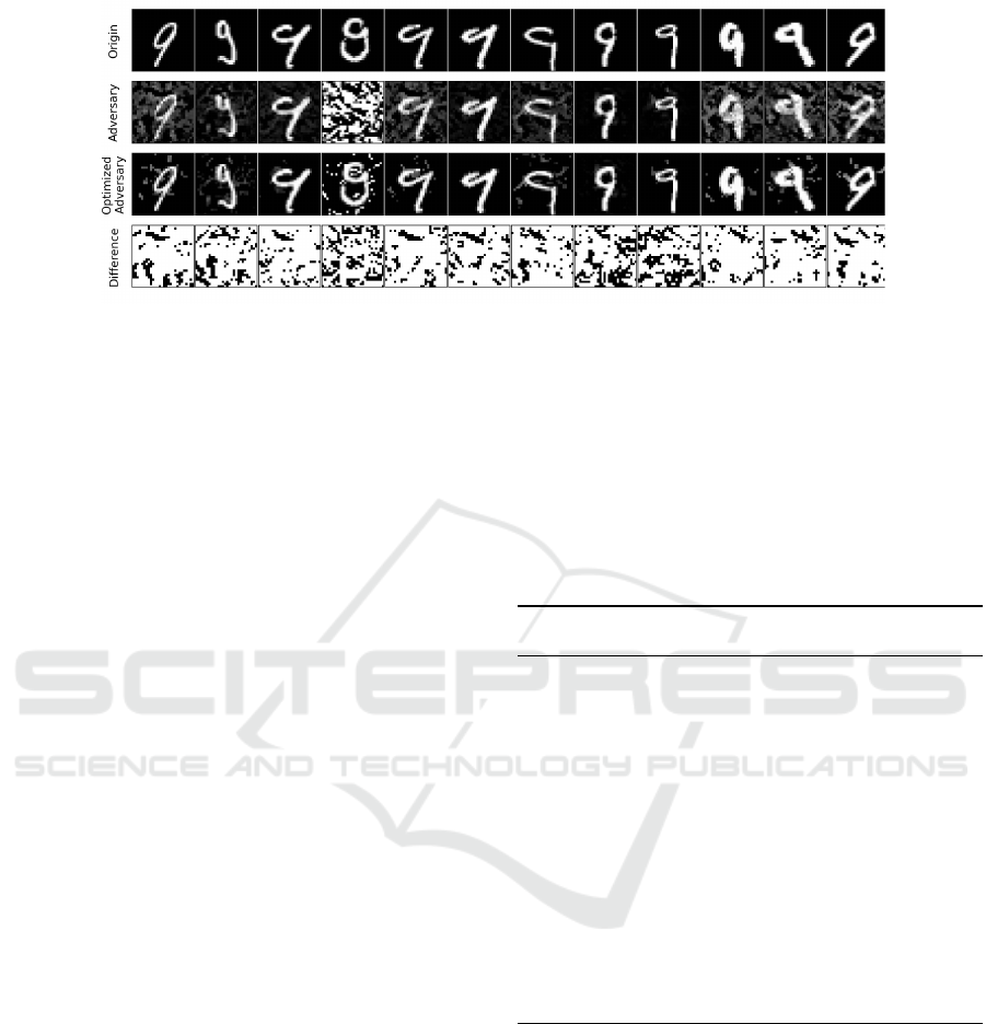
Figure 1: A motivating example.

ATN (Baluja and Fischer, 2017) are common meth-

ods. We observed that the quality of the adversar-

ial example generated by these methods could be en-

hanced more in terms of L

-norm and L

-norm.

Figure 1 shows a motivating example of this re-

search. The ﬁrst row Origin shows the original im-

ages which are modiﬁed to produce adversarial exam-

ples. The second row Adversary contains adversar-

ial examples generated by applying box-constrained

L-BFGS. The third row shows the optimized adver-

sary. The last row represents the difference between

the second row and the third row. White pixel denotes

the difference and dark pixel is corresponding to iden-

ticalness.

As can be seen, by comparing the second row and

the third row, some optimized adversarial examples

are very different from the corresponding adversarial

examples. In other words, the adversarial examples

in the second row still contain many redundant per-

turbations. To minimize L

-norm and L

-norm, these

redundant perturbations should be recognized and re-

moved from the adversarial examples. Therefore, this

paper proposes a method to enhance the quality of

adversarial examples generated by any adversarial at-

tacks with low computational cost. We focus on L

norm and L

-norm.

4 GREEDY METHOD

To the best of our knowledge, there is no similar work

to improve the quality of adversarial examples gen-

erated by adversarial attacks. Most of the research

on this topic aims to generate high-quality adversar-

ial examples during the adversarial attack, not after

the adversarial attack. Therefore, to show the effec-

tiveness of the proposed method, this research com-

pares it with a greedy approach. We also explain why

although the greedy method could produce good re-

sults of adversary improvement, it has several prob-

lems when applying in practice.

Algorithm 1 describes the overview of the greedy

method to enhance the quality of an adversarial exam-

ple. The input includes an adversarial examples x

, its

corresponding input image x, an attacked model M,

and a step α. The target label is the predicted label

of x

. The output is an improved adversarial exam-

ple. The greedy method is used as a baseline in the

experiments.

Algorithm 1: Greedy Method: Improve the quality of ad-

versarial examples in terms of L

-norm and L

-norm.

Input: adversarial example x

, input image x, DNN M,

step α

Output: An improved adversarial example

1: l = argmax(M(x

))

2: while α > 0 do

3: F

adv

← GET-ADVERSARIAL-FEATURES(x, x

)

4: B

adv

= F

0..α−1

α..2∗α−1

...

n∗α..kF

adv

5: for F

i.. j

∈ B

adv

6: x

= Update x

← x

, ..., x

← x

7: if argmax(M(x

)) 6= l then

8: Undo the step 6

9: end if

10: end for

11: α ← bα/2c

12: end while

13: return x

In the greedy method, a set of adversarial features

(denoted by F

adv

) is detected by comparing x

and x

(line 3). The order of adversarial features is arranged

from the top left corner to the bottom right corner of

. The greedy method attempts to restore the adver-

sarial features on this set to the original values. The

original value of adversarial feature x

is x

. We use a

step (denoted by α >= 1) to determine the number of

adversarial features restored at the same time.

The greedy method speciﬁes subsets of adversar-

ial features by dividing the set F

adv

(line 4). Subset

i.. j

stores the adversarial features from i

position

Method for Improving Quality of Adversarial Examples

217

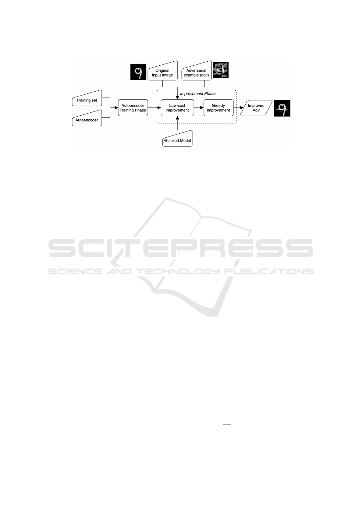
Figure 2: The overview of the proposed method.

to j

position on F

adv

. After that, we iterate over

these subsets. At each iteration, the adversarial fea-

tures from i

position to j

position on x

attempts

to be restored to the original values (line 6). There

are two cases. If this restoration changes the label of

(line 7 - 8), the modiﬁcation on x

is reverted to

preserve its predicted label. Otherwise, the modiﬁca-

tion on x

is kept. The algorithm moves to the next

subset of F

adv

When more adversarial features are restored at the

same time, the probability to change the decision of

the attacked model on x

is larger. Therefore, after

iterating all subsets F

i.. j

, the step α decreases by twice

(line 11). The algorithm performs the restoration of

adversarial features with a smaller size of subset F

i.. j

The algorithm terminates when α is not greater than 1.

However, the greedy method has two main limi-

tations. Firstly, the greedy method does not support

the generalization ability. The experiences of improv-

ing an adversarial example in the past are not utilized

to enhance new adversarial examples. Secondly, this

method has poor performance. The total cost of ex-

ecuting line 7 could be time-consuming. The DNN

model predicts the label of the temporary modiﬁca-

tion of an adversarial example. It requires the ini-

tialization of DNN, many computations on the DNN

graph to obtain a result. Especially, this cost could

be huge when the number of redundantly adversar-

ial features is large. For example, in FGSM, most of

the features on an input image would be modiﬁed to

generate an adversarial example. It means that more

number iterations (i.e., line 5) would be performed.

5 THE PROPOSED METHOD

This paper proposes a method to mitigate the limita-

tion of the greedy method. The overview of the pro-

posed method is illustrated in Fig. 2. The proposed

method includes two main phases, namely autoen-

coder training phase and improvement phase. The

purpose of the autoencoder training phase is to train

an autoencoder, which is an input of the second phase.

The purpose of the improvement phase is to enhance

the quality of adversarial examples in terms of L

norm and L

-norm distance.

5.1 Autoencoder Training Phase

The input of this phase includes the training set and

the architecture of an autoencoder denoted by g. The

output of this phase is a trained autoencoder.

The training set is a set of (x

), where x

∈ R

is an unimproved adversarial example and s

∈ R

a 0-1 vector. Each value s

[i] represents the probabil-

ity to restore the adversarial feature x

[i] to the original

values:

[i] =



1 if x

is redundant

0 otherwise

(8)

For example, consider an unimproved adversarial

example x

= [0, 0,1,...,0.5, 0]

∈ R

784

. The corre-

sponding input image of this adversarial example is

x = [1,0,1, ...,0.5,0]

∈ R

784

. Restoring the adver-

sarial feature x

(i.e., value 0) to the original value

(i.e., value 1) produces a modiﬁed adversarial exam-

ple. If the label of the modiﬁed adversarial example

is the same as that of x

, x

is redundant. Therefore,

[0] is assigned to 1. Otherwise, s

[0] is assigned

to 0.

The architecture of the autoencoder g is deﬁned

manually. The output of the autoencoder from an ad-

versarial example x

is denoted by g(x

). For an ad-

versarial example x

on the training set, the objective

of the autoencoder is deﬁned as follows:

|−1

∑

i=0

f (s

[i],g(x

)[i])

(9)

where f is binary cross-entropy.

ICAART 2022 - 14th International Conference on Agents and Artiﬁcial Intelligence

218

The proposed autoencoder in Equation 9 is differ-

ent from the traditional autoencoder. The main dif-

ference is the output g(x

) of the autoencoder. In the

traditional autoencoder, g(x

) should be identical to

the input x

. In this case, the metric mean squared er-

ror is usually used to measure the distance between

and g(x

). However, in our proposed autoencoder,

g(x

) is a probability vector. Therefore, we use binary

cross-entropy to compare g(x

) and s

5.2 Improvement Phase

This phase improves the quality of adversarial exam-

ples in terms of L

-norm and L

-norm. The input

of this phase is an attacked model M, a trained au-

toencoder g (i.e., the result of the previous phase),

an unimproved adversarial example x

, and its corre-

sponding input image x. The output of this phase is

an improved adversarial example. This phase has two

main steps including a low-cost improvement step and

a greedy improvement step.

Low-cost Improvement Step. In this step, the

trained autoencoder g is used to generate the ﬁrst ver-

sion of the improved adversarial example, denoted by

. Because g(x

) is a probability vector, we need

a threshold δ ∈ [0,1] to determine whether g(x

)[i] is

classiﬁed as redundant or not. The ﬁrst version x

created as follows:

[i] =



if g(x

)[i] <= δ

otherwise

(10)

The ﬁrst version x

is then predicted by the at-

tacked model M. If the label of x

is the same as that

of x

, x

is then fed into the second step of this phase.

Otherwise, the value of threshold δ should increase.

When δ increases, there is fewer number of redun-

dantly adversarial features. As a result, x

is more

close to x

. The attacked model M tends to predict the

label of x

and x

the same.

The low-cost improvement step takes low compu-

tational cost. The experiment has shown that this au-

toencoder takes around 1-2 seconds for the MNIST

dataset (Lecun et al., 1998a) and around 3-4 sec-

onds for the CIFAR-10 dataset (Krizhevsky, 2012) for

about 1,000 adversarial examples.

Greedy Improvement Step. It is observed that the

ﬁrst version x

could be enhanced more. There are

some adversarial features on x

that could be re-

stored to the original values. Therefore, the pro-

posed method applies the greedy method described in

Sect. 4 to ﬁnd out such adversarial features. The out-

put of this step is the second version of the improved

adversarial example, denoted by x

. The proposed

method returns x

as the ﬁnal improved adversarial

example of x

and terminates.

6 EXPERIMENTAL RESULTS

To demonstrate the advantages of the proposed

method, the experiments address the following ques-

tions:

• RQ1 - Success Rate of Autoencoder: Does the

trained autoencoder improve most of the adversar-

ial examples?

• RQ2 - Quality: Does the proposed improvement

phase reduce the L

-norm and L

-norm of the

unimproved adversarial examples?

• RQ3 - Performance: Does the proposed im-

provement phase achieve good performance when

dealing with the unimproved adversarial exam-

ples?

For the autoencoder training phase, we answer

RQ1 to investigate the effectiveness of the trained au-

toencoders. For the improvement phase, the experi-

ments answer RQ2 and RQ3 by comparing this phase

with the greedy method. The experiments are per-

formed on Google Colab

6.1 Conﬁguration

6.1.1 Dataset

The experiments are conducted on the

MNIST dataset (Lecun et al., 1998a) and the

CIFAR-10 (Krizhevsky, 2012) dataset. These

datasets are used commonly to evaluate the robust-

ness of DNN models (Zhang et al., 2019). About

the MNIST dataset, it is a collection of handwritten

digits. The training set has 60,000 images and the

test set contains 10,000 images of size 28 × 28 ×

1. There are 10 labels representing the digits from

0 to 9. Concerning the CIFAR-10 dataset, it is a

collection of images labelled as aeroplanes, trucks,

birds, cats, etc. It has 50,000 images on the training

set and 10,000 images of size 32 × 32 × 3 on the test

set. One pixel is described in a combination of red,

green, and blue channels.

6.1.2 Attacked Model

For the MNIST dataset, the experiments use

LeNet-5 (Lecun et al., 1998b). This architec-

ture is introduced to recognize handwritten dig-

its. For the CIFAR-10 dataset, the experiments use

https://colab.research.google.com/

Method for Improving Quality of Adversarial Examples

219

AlexNet (Krizhevsky et al., 2017). Compared to the

architecture of LeNet-5, the architecture of AlexNet

is more complicated. This model is used for general-

purpose image classiﬁcation. The accuracies of the

trained models are shown in Table 1.

Table 1: The accuracy of attacked models.

Dataset Model Training set Test set

MNIST LeNet-5 99.86% 98.82%

CIFAR-10 AlexNet 99.70% 76.22%

6.1.3 Adversarial Example

The adversarial examples are generated by apply-

ing three adversarial attacks including FGSM, box-

constrained L-BFGS, and ATN. The purpose is to

demonstrate the effectiveness of the proposed method

when dealing with various adversarial examples. For

FGSM and L-BFGS, the experiments use their orig-

inal equations. For ATN, we make several small

modiﬁcations in Equation 6 to generate more high-

quality adversarial examples. We empirically use

cross-entropy instead of L

-norm to compare the dis-

tance between the expected probability and the pre-

dicted probability. Additionally, we use the identity

function instead of the reranking function.

If the original input images labelled m are mod-

iﬁed into an adversarial example classiﬁed as n, the

experiments denote as the attack m → n for simplic-

ity. For the MNIST dataset, the attack is 9 → 4. For

the CIFAR-10 dataset, the attack is truck → horse.

6.1.4 The Proposed Method

Autoencoder Training Phase. In the ﬁrst phase of

the proposed method, we train autoencoders to recog-

nize redundant perturbations existing inside an adver-

sarial example. Each autoencoder is trained on 6,000

samples by using the Equation 9. A sample is a set

of (x

), where x

is unimproved adversarial exam-

ples. These training sets are denoted by X

train

. These

autoencoders are trained in 300 epochs.

The architectures of autoencoders should be de-

ﬁned based on the experience of machine learning

testers. The experiments use stacked convolutional

autoencoders because these autoencoders could learn

the characteristics of 2D and 3D images better than

traditional autoencoders. Table 2 describes the gen-

eral architecture of the autoencoders used in the pro-

posed method. The architectures of these autoen-

coders are the same, except for the input layer and the

output layer. The layer before the output layer uses

sigmoid to compute the probability for binary classi-

ﬁcation.

Table 2: The architectures of the autoencoders used in the

proposed method. For MNIST, the shape of input is (28,

28, 1). For CIFAR-10, the shape of input is (32, 32, 3).

Layer Type Conﬁguration

Input #width × #height × #channel

Conv2D + ReLU kernel = (3, 3), #ﬁlters = 64

BatchNormalization

MaxPooling pool˙size = (2, 2)

Conv2D + ReLU kernel = (3, 3), #ﬁlters = 32

BatchNormalization

MaxPooling2D pool˙size = (2, 2)

Conv2D + ReLU kernel = (3, 3), #ﬁlters = 32

BatchNormalization

UpSampling2D pool˙size = (2, 2)

Conv2D + ReLU kernel = (3, 3), #ﬁlters = 64

BatchNormalization

UpSampling2D pool˙size = (2, 2)

Conv2D + Sigmoid kernel = (3, 3), #ﬁlters = #channel

Output #width × #height × #channel

Improvement Phase. The experiments use 1,000 ad-

versarial examples denoted by X

test

to evaluate the ef-

fectiveness of the proposed method. These adversar-

ial examples are not used to train autoencoders. The

conﬁguration of improvement is as follows:

• Low-cost Improvement Step. Unimproved ad-

versarial examples are fed into the trained autoen-

coders.

• Greedy Improvement Step. For MNIST, the

value of step α (in Algorithm 2) is 6. While the

number of features on CIFAR-10 is much larger

than that of MNIST, the initial value of step α for

CIFAR-10 should be larger. For CIFAR-10, we

empirically assign the initial value of step α to 60.

6.1.5 Baseline

The proposed method is compared with the greedy

method. It is the baseline in the experiment. The in-

put of the baseline is 1,000 unimproved adversarial

examples. These adversarial examples are the same

as the adversarial examples used in the improvement

phase of the proposed method.

Additionally, the conﬁguration α of the baseline

is the same as the greedy improvement step in the

proposed method. Speciﬁcally, for MNIST, the ini-

tial value of step α is 6. For CIFAR-10, the initial

value of step α is 60.

ICAART 2022 - 14th International Conference on Agents and Artiﬁcial Intelligence

220

6.2 Answer for RQ1 - Success Rate of

Autoencoder

This section investigates the success rate of the au-

toencoders. These autoencoders are trained on X

train

consisting of around 6,000 samples and evaluated on

test

consisting of about 1,000 samples. The success

rate is the percentage of the unimproved adversarial

examples which are enhanced successfully by the au-

toencoders. If the success rate is close to 100%, most

unimproved adversarial examples are enhanced their

quality by the trained autoencoders.

We observed that increasing threshold δ in Equa-

tion 10 would increase the success rate. The main rea-

son is that when the value of δ goes up, there is less

number of adversarial features restored to the orig-

inal values. In other words, the modiﬁed adversar-

ial example is closer to the unimproved adversarial

example. As a result, the label of the modiﬁed ad-

versarial example tends to be the same as that of the

unimproved adversarial example. For example, Fig. 3

describes the impact of threshold on the success rate.

As can be seen, the success rate increases to nearly

100% when δ goes up to nearly 1.

Figure 3: Trend of success rate when using different thresh-

olds. The adversarial examples are generated by FGSM.

The attacked model is LeNet-5 trained on MNIST.

The experiments continue investigating more

deeply the impact of three values of δ including 0.93,

0.96, and 0.99 on success rate. The main reason of

using these δ is that it would result in high success

rate. We compute the average success rate rather

than reporting the success rate of each threshold in-

dividually. Table 3 shows the average success rate of

the trained autoencoders. For example, 97.2% means

the trained autoencoders could improve the quality of

about |X

train

| × 97.2% adversarial examples. As can

be seen, the trained autoencoders could enhance the

quality of most adversarial examples on X

train

, from

around 87% to about 97%. For X

test

, the success rates

are from around 81% to about 90%. This shows that

the trained autoencoders can recognize redundant per-

turbation inside adversarial examples effectively.

Table 3: Average success rate of the trained autoencoders.

Dataset Method Training set Test set

MNIST

FGSM 97.2% 90.4%

L-BFGS 89.3% 87.1%

ATN 95.2% 92.2%

CIFAR-10

FGSM 87.4% 81.3%

L-BFGS 87.3% 83.3%

ATN 87.7% 86.4%

The trained autoencoders in RQ1 are used to an-

swer RQ2 and RQ3. These two research questions

only evaluate the effectiveness of the improvement

phase. Given the same subset of unimproved ad-

versarial examples, the experiments investigate if the

proposed improvement phase works better than the

greedy method. Two compared metrics are the reduc-

tion rate of L

-norm and the performance.

6.3 Answer for RQ2 - Quality

Improvement

This section demonstrates how the proposed improve-

ment phase enhances the quality of X

test

in terms

of L

-norm and L

-norm. These adversarial exam-

ples are not used to train the autoencoder. The com-

pared method is the greedy method. The compared

metric is the reduction rate, which is computed by

(a − b)/a ∈ [0, 1), where a is the distance before the

improvement, b is the distance after the improvement.

It is expected that b should be as small as possible.

In the proposed improvement phase, the process

of improving adversarial examples is as follows. In

the ﬁrst step, X

test

is fed into the low-cost improve-

ment step. The improved adversarial examples are

the ﬁrst version of the improvement. In the second

step, the output of the ﬁrst step is fed into the greedy

improvement step to enhance its quality more.

In the low-cost improvement step, the parameter

δ of the trained autoencoders should be chosen to im-

prove the quality of X

test

as much as possible. We

empirically observed that δ ∈ [0.8,1) would result in

good reduction rate of L

-norm and L

-norm. For

example, Fig. 4 describes the impact of threshold δ

on the reduction rate of L

-norm and L

-norm. As

can be seen, increasing the threshold δ to around 0.9x

improves the reduction rate of both L

-norm and L

norm signiﬁcantly. The reduction rates then decrease

slightly when δ is very close to 1.

Based on the above observation, the experiments

Method for Improving Quality of Adversarial Examples

221

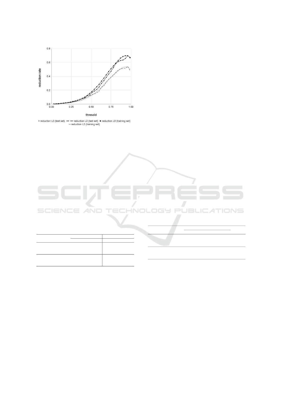
Figure 4: Trend of reduction rate when using different

thresholds δ. The adversarial examples are generated by

FGSM. The attacked model is LeNet-5 trained on MNIST.

choose δ used in RQ1 (i.e., 0.93, 0.96, and 0.99)

to make comparison with the greedy method. Ta-

ble 4 shows the average reduction rate of L

-norm

and L

-norm. Generally, the proposed improvement

phase produces better results than the greedy method

in 8/12 cases. The experiment shows that the pro-

posed improvement phase could achieve the reduction

rate from around 82% to about 95% in terms of L

norm. Concerning L

-norm, the reduction rate of the

proposed improvement phase is from around 56% to

approximately 81%.

Table 4: The average reduction rate (%) of L

-norm and L

norm on X

test

. Better values are bold. Notion * means that

we ignore the process of training autoencoder.

-norm L

-norm

Dataset Method

Proposal*

Greedy

Proposal*

Greedy

FGSM 82.58 82.40 68.91 68.07

L-BFGS 82.38 82.30 68.01 72.79MNIST

ATN 95.20 94.27 59.67 56.77

FGSM 85.27 84.92 81.07 79.31

L-BFGS 83.90 87.14 63.8 66.54CIFAR-10

ATN 86.45 88.69 68.27 66.09

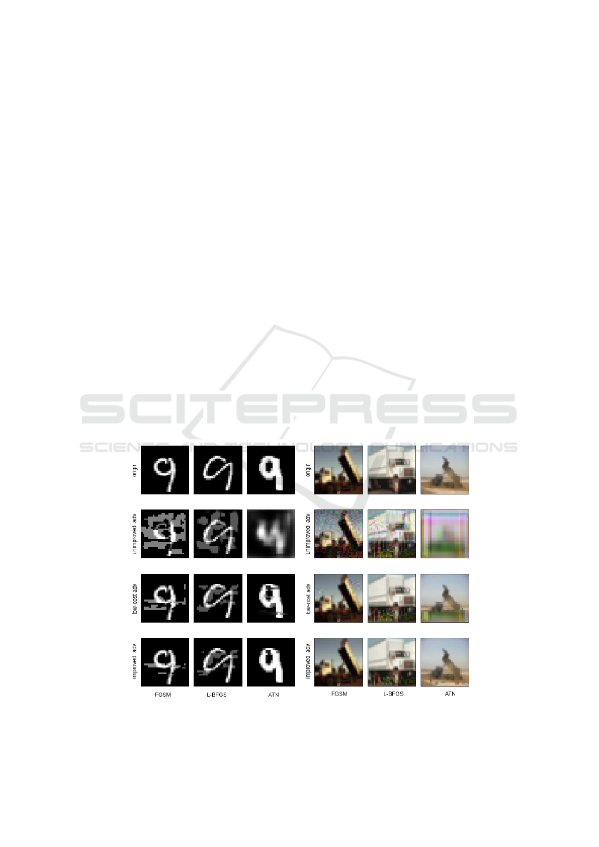
Figure 5 shows some examples of the improved

adversarial examples by applying the proposed im-

provement phase. Row origin represents the input

images, which are modiﬁed to generate adversarial

examples. The result of adversarial attacks on these

input images is stored in the second row unimproved

adv. The adversarial examples in this row are not im-

proved by applying the proposed improvement phase.

The third row low-cost adv shows the ﬁrst version

of the improved adversarial examples. This row is

the result of applying the low-cost improvement step.

The last row improved adv shows the result of ap-

plying the greedy method. The ﬁrst version of the

improved adversarial examples is fed into the greedy

method to generate more high-quality results. As can

be seen, in terms of human perception, the low-cost

improvement step could enhance the quality of unim-

proved adversarial examples signiﬁcantly. However,

there are some redundantly adversarial perturbations

in the third row. By applying the greedy improvement

step, such perturbations are detected and removed.

6.4 Answer for RQ3 - Performance

This section evaluates the performance of the pro-

posed improvement phase when dealing with X

test

These adversarial examples are used in RQ2. This

experiment uses different values of threshold δ (i.e.,

0.93, 0.96, and 0.99) as discussed in RQ1 and RQ2.

Table 5 shows the performance comparison in sec-

onds between the proposed improvement phase and

the greedy method. The computational cost of the

proposed improvement phase includes the low-cost

improvement step and the greedy improvement step.

In the low-cost improvement step, X

test

are fed into

the trained autoencoders to retrieve the ﬁrst version

of the improved adversarial examples. However, we

observed that these improved adversarial examples

could be enhanced more in terms of L

-norm and L

norm. Therefore, these improved adversarial exam-

ples are put into the greedy improvement step to ob-

tain the second version of improvement.

Table 5: The average performance comparison (seconds)

between the proposed improvement phase and the greedy

method on the test set. Better values are bold.

Proposed improvement phase

Dataset Method

Low-cost Greedy

∑

Greedy

FGSM 1.1 13.1 14.2 80.3

L-BFGS 1.2 27.6 28.8 98.3MNIST

ATN 1.4 20.1 21.5 120.2

FGSM 3.7 29.1 32.8 250.8

L-BFGS 3.5 46.1 49.6 261.1CIFAR-10

ATN 3.4 62.1 65.5 254.5

As can be seen, the performance of the proposed

improvement phase outperforms that of the greedy

method. On the MNIST dataset, the proposed im-

provement phase usually requires from around 14.2

seconds to about 28.8 seconds, which is from roughly

3 times faster to around 6 times faster than that of the

greedy method. On the CIFAR-10 dataset, the time of

the proposed improvement phase is approximately 4

times to 8 times faster than that of the greedy method.

The main reason is that in the proposed improvement

phase, most of the adversarial features are restored

to the original values by applying the trained autoen-

coders. As a result, there is only a small set of re-

dundant features restored by the greedy improvement

step. This helps to reduce the cost of the greedy im-

ICAART 2022 - 14th International Conference on Agents and Artiﬁcial Intelligence

222

provement step, which is a time-consuming process.

Combining the result of research questions, the

experiments show three insights. The ﬁrst insight is

that the proposed improvement phase could improve

the quality of most adversarial examples. The second

result is that the proposed improvement phase could

improve the quality of new adversarial examples con-

siderably. The third insight is that the proposed im-

provement phase has a low computational cost when

dealing with new adversarial examples.

7 RELATED WORK

This section presents an overview of related research.

Firstly, we discuss some well-known adversarial at-

tacks using L

-norm metric. Secondly, we clarify

the novelty of the proposed method by discussing the

state of adversarial example improvement methods.

Adversarial Example Generation. Many adver-

sarial example generation methods are introduced to

evaluate the robustness of DNNs. These methods add

perturbations to an input image to generate an ad-

versarial example. Several common methods are de-

scribed as follows.

Box-constrained L-BFGS (Szegedy et al., 2014)

minimizes L

-norm by proposing an objective func-

tion for each input image. This objective ensures that

the modiﬁcation of an input image is small while it

is classiﬁed as a target label. However, this method

does not treat the complex DNNs well because of the

highly nonlinear property of the objective function.

Similarly to box-constrained L-BFGS, DeepFool

(Moosavi-Dezfooli et al., 2015) aims to generate ad-

versarial examples with small L

-norm. This method

assumes that the network to be completely linear.

They compute a solution on the tangent plane (orthog-

onal projection) of a point on the classiﬁer function.

However, DNNs are not linear, this method then takes

a step towards that solution, and repeats the process.

The search terminates when an adversarial example is

found.

FGSM (Goodfellow et al., 2015) adds perturba-

tion to all features. This method has a low computa-

tional cost. However, the generated adversarial exam-

ples usually contain visible noises, which is not real-

istic in practice. Additionally, the L

∞

-norm distance

is sensitive to the value of the input parameter.

Carnili-Wagner (Carlini and Wagner, 2016) im-

proves the box-constrained L-BFGS by reducing the

highly nonlinear property of the objective function.

They apply the change of variable technique and use

a simpler objective function. Their experiments have

shown that the perturbation is much smaller than box-

constrained L-BFGS.

Unlike the above methods, ATN (Baluja and Fis-

cher, 2017) trains autoencoder for adversarial attack.

The autoencoder could be used to generate adversar-

(a) MNIST (b) CIFAR-10

Figure 5: Examples of the improved adversarial examples by the proposed improvement phase.

Method for Improving Quality of Adversarial Examples

223

ial examples from new input images with a low com-

putational cost. Their method has the generalization

ability, which is not supported by most of the exist-

ing methods.

DeepCheck (Gopinath et al., 2019) is the ﬁrst

symbolic execution tool for testing DNNs. This

method translates a DNN into a Java program. From

an input image, the program is instrumented and exe-

cuted to get the execution path. After that, symbolic

execution is applied on this path to obtain path con-

straints. These path constraints are modiﬁed by ﬁxing

a set of features. The modiﬁed constraints are solved

by using an SMT-Solver such as Z3 (De Moura and

Bjørner, 2008) to get a solution. This method could

generate an adversarial example with a very small L

norm. However, this method consumes a large com-

putational cost due to the symbolic execution and the

usage of SMT-Solvers.

Adversarial Example Improvement. To the best

of our knowledge, most works in this ﬁeld do not

consider the improvement of adversarial examples as

an independent phase. Instead, they add the objec-

tive of L

-norm minimization to the objective func-

tion such as box-constrained L-BFGS (Szegedy et al.,

2014), Carnili-Wagner (Carlini and Wagner, 2016),

ATN (Baluja and Fischer, 2017), etc. Our method

could be considered as the second phase of the ad-

versarial example generation methods. The proposed

method could be used to enhance the quality of adver-

sarial examples generated by any attack.

8 CONCLUSION

We have presented a method to improve the qual-

ity of adversarial examples in terms of L

-norm and

-norm. The proposed method includes two phases

namely the autoencoder training phase and the im-

provement phase. In the autoencoder training phase,

the proposed method trains an autoencoder to learn

how to detect redundantly adversarial features. In

the improvement phase, the autoencoder improves the

quality of a new adversarial example to generate the

ﬁrst version of the improvement. After that, the ﬁrst

improvement version is fed into the greedy improve-

ment step to enhance more. The experiments are

conducted on the MNIST dataset and the CIFAR-10

dataset. The proposed method could enhance the L

norm and L

-norm signiﬁcantly. Additionally, the

proposed method could improve the quality of new

adversarial examples with a low computational cost.

It means that the proposed method could be applied

in practice.

In the future, we would investigate more deeply

the impact of high-quality adversarial examples on

the performance of the adversarial defence. Be-

sides, we would evaluate the effectiveness of the pro-

posed method with different kinds of autoencoder

such as denoising autoencoder, sparse autoencoder,

variational autoencoder, symmetric autoencoder, etc.

Finally, we would investigate the effectiveness of

the proposed method with the adversarial examples

generated by other methods such as Carnili-Wagner,

DeepFool, DeepCheck, etc.

ACKNOWLEDGEMENTS

This work has been supported by VNU University

of Engineering and Technology under project number

CN21.09.

Duc-Anh Nguyen was funded by Vingroup JSC

and supported by the Master, PhD Scholarship Pro-

gramme of Vingroup Innovation Foundation (VINIF),

Institute of Big Data, code VINIF.2021.TS.105.

Kha Do Minh was funded by Vingroup JSC

and supported by the Master, PhD Scholarship Pro-

gramme of Vingroup Innovation Foundation (VINIF),

Institute of Big Data, code VINIF.2021.ThS.24.

REFERENCES

Baluja, S. and Fischer, I. (2017). Adversarial transformation

networks: Learning to generate adversarial examples.

Carlini, N. and Wagner, D. A. (2016). Towards eval-

uating the robustness of neural networks. CoRR,

abs/1608.04644.

Ciregan, D., Meier, U., and Schmidhuber, J. (2012). Multi-

column deep neural networks for image classiﬁcation.

In 2012 IEEE Conference on Computer Vision and

Pattern Recognition, pages 3642–3649.

De Moura, L. and Bjørner, N. (2008). Z3: An efﬁcient smt

solver. In Proceedings of the Theory and Practice of

Software, 14th International Conference on Tools and

Algorithms for the Construction and Analysis of Sys-

tems, TACAS’08/ETAPS’08, pages 337–340, Berlin,

Heidelberg. Springer-Verlag.

Eniser, H. F., Gerasimou, S., and Sen, A. (2019). Deepfault:

Fault localization for deep neural networks. CoRR,

abs/1902.05974.

Goodfellow, I. J., Shlens, J., and Szegedy, C. (2015). Ex-

plaining and harnessing adversarial examples.

Gopinath, D., P

areanu, C. S., Wang, K., Zhang, M., and

Khurshid, S. (2019). Symbolic execution for attribu-

tion and attack synthesis in neural networks. In Pro-

ceedings of the 41st International Conference on Soft-

ware Engineering: Companion Proceedings, ICSE

’19, page 282–283. IEEE Press.

ICAART 2022 - 14th International Conference on Agents and Artiﬁcial Intelligence

224

Krizhevsky, A. (2012). Learning multiple layers of features

from tiny images. University of Toronto.

Krizhevsky, A., Sutskever, I., and Hinton, G. E. (2017). Im-

agenet classiﬁcation with deep convolutional neural

networks. Commun. ACM, 60(6):84–90.

Kurakin, A., Goodfellow, I. J., and Bengio, S. (2016).

Adversarial examples in the physical world. CoRR,

abs/1607.02533.

Lecun, Y., Bottou, L., Bengio, Y., and Haffner, P. (1998a).

Gradient-based learning applied to document recogni-

tion. In Proceedings of the IEEE, pages 2278–2324.

Lecun, Y., Bottou, L., Bengio, Y., and Haffner, P. (1998b).

Gradient-based learning applied to document recogni-

tion. Proceedings of the IEEE, 86(11):2278–2324.

Moosavi-Dezfooli, S., Fawzi, A., and Frossard, P. (2015).

Deepfool: a simple and accurate method to fool deep

neural networks. CoRR, abs/1511.04599.

Sultana, F., Suﬁan, A., and Dutta, P. (2019). Advancements

in image classiﬁcation using convolutional neural net-

work. CoRR, abs/1905.03288.

Szegedy, C., Zaremba, W., Sutskever, I., Bruna, J., Erhan,

D., Goodfellow, I., and Fergus, R. (2014). Intriguing

properties of neural networks.

Zhang, J., Harman, M., Ma, L., and Liu, Y. (2019). Machine

learning testing: Survey, landscapes and horizons.

Method for Improving Quality of Adversarial Examples

225