Learning Heuristic Estimates for Planning in Grid Domains by Cellular

Simultaneous Recurrent Networks

Michaela Urbanovsk

a and Anton

ın Komenda

Department of Computer Science (DCS), Faculty of Electrical Engineering (FEE),

Czech Technical University in Prague (CTU), Karlovo namesti 293/13, Prague, 120 00, Czech Republic

Keywords:

Classical Planning, Simultaneous Recurrent Neural Networks, Heuristic Learning, Deep Learning.

Abstract:

Automated planning provides a powerful general problem solving tool, however, its need for a model cre-

ates a bottleneck that can be an obstacle for using it in real-world settings. In this work we propose to use

neural networks, namely Cellular Simultaneous Recurrent Networks (CSRN), to process a planning problem

and provide a heuristic value estimate that can more efﬁciently steer the automated planning algorithms to

a solution. Using this particular architecture provides us with a scale-free solution that can be used on any

problem domain represented by a planar grid. We train the CSRN architecture on two benchmark domains,

provide analysis of its generalizing and scaling abilities. We also integrate the trained network into a planner

and compare its performance against commonly used heuristic functions.

1 INTRODUCTION

Classical planning is a powerful tool in terms of gen-

eral problem solving. Its performance relies heavily

on heuristic functions which provide further informa-

tion about the problem and suggest which states to ex-

pand in search of the solution. There are many widely

used heuristic functions that provide informed state-

goal distance estimate, however, to compute such es-

timate we need to model the problem we try to solve.

Problem representation for classical planning of-

ten has to be done by hand and some problems can be

too hard to describe and model in standardized lan-

guages such as PDDL (Aeronautiques et al., 1998).

That creates a bottleneck which complicates usage

of classical planning techniques on complex or very

large domains that are too hard to be modeled by a hu-

man. That holds for many real-world problems such

as logistic problems, distribution warehouses or fork-

lift ﬂeets.

One way to avoid creating such representation is

using a graphical representation of the problem. In

conjunction with neural networks we take the mod-

elling part out of the equation and base the heuris-

tic computation on graphical features and not a hand-

coded model.

Combining classical planning with neural net-

works is currently widely discussed problem which

is being tackled from many different perspectives.

In (Shen et al., 2020), authors use hypergraph neu-

ral networks together with the standardized modelling

language to compute heuristic value for a given state.

In (Groshev et al., 2018) the authors take similar path

to ours where they use graphic representation of the

problem and compute a policy which should be fol-

lowed in the search algorithm.

Another approach which uses image representa-

tion is (Asai and Fukunaga, 2017) and (Asai and

Fukunaga, 2018) where authors convert the image

into latent space and further evaluate it using neural

networks to obtain a heuristic.

One type of neural networks which have been suc-

cessful with problems represented by an image-like

grid are the Cellular Simultaneous Recurrent Net-

works (CSRN). In particular, they were used to solve

the maze traversal problem. As mentioned in (Ilin

et al., 2008), output of the network can be used to

greedily guide an algorithm from a start state to a goal

using values generated by the network as a heuristic

function which means that it can be used in classi-

cal planning algorithms. There are works regarding

the CSNR architecture such as (Ilin et al., 2006) and

(White et al., 2010) which mostly focused on improv-

ing its training which is a great bottleneck of this ap-

proach.

In this work, we implemented CSRN for both

maze and Sokoban domains based on implementa-

tion in (Ilin et al., 2008). We analyze training of the

Urbanovská, M. and Komenda, A.

Learning Heuristic Estimates for Planning in Grid Domains by Cellular Simultaneous Recurrent Networks.

DOI: 10.5220/0010813900003116

In Proceedings of the 14th International Conference on Agents and Artiﬁcial Intelligence (ICAART 2022) - Volume 2, pages 203-213

ISBN: 978-989-758-547-0; ISSN: 2184-433X

203

CSRN architecture, discuss the parameters, training

and evaluation. At the same time, we focus on its

ability to generalize over different problem instances

and discuss how to use it as a domain-independent

heuristic function. At last, we integrate the CSRN in a

classical planner and compare its performance against

other heuristic functions.

2 BACKGROUND

Classical planning is a form of general problem solv-

ing that starts in a fully deﬁned initial state and looks

for a goal state by applying deterministic actions.

For each problem we need a set of facts which cre-

ate the states and a set of actions which can be applied

to said states. The two sets form a graph which can

be referred to as a state-space of the problem. In this

state-space we then look for a solution using state-

space search algorithms.

2.1 State-space Search

Any search algorithm starts at the initial state and in

each step applies all applicable actions to create more

states which are further expanded until a goal state is

reached. We can then reconstruct the path leading to

solution by taking every expansion that led to the goal

state from the beginning of the algorithm.

Such graph traversal algorithm can be computed

blindly and states can be expanded in ﬁrst-in ﬁrst-out

manner as a breadth-ﬁrst search (Bundy and Wallen,

1984). However, the state-spaces tend to be large and

exhaustive search may not be the most efﬁcient way

to ﬁnd the solution. The performance of a search al-

gorithm can be improved by using a heuristic function

to guide it. There are many state-space search algo-

rithms which use a heuristic function. In this work,

we use Greedy Best-ﬁrst Search (GBFS) which relies

solely on the heuristic function when making a deci-

sion. Because we use a neural network to estimate

the heuristic value and we have no guarantees on the

generated heuristic values, we use GBFS in our ex-

periments.

2.2 Heuristic Functions

Heuristic function is a function h(s) → R

that takes

a state s on the input and returns a single value that

estimates how far is the given state from a goal. Based

on the values provided by the heuristic function, the

search can make much more informed decisions in

which state to expand next.

In this work, we use multiple different heuristic

functions in the experiments to compare their perfor-

mance. The most simple heuristic is a blind heuris-

tic, which gives each estimate equal to zero. Next

used heuristic function is Euclidean Distance (ED)

which computes Euclidean distance from current state

to goal state on a grid. These two heuristics are very

fast and simple to compute, but the information they

add to the search may not be very valuable.

Another heuristics, we use in the experiments,

are h

(Hoffmann, 2001) and LM-cut (Pommeren-

ing and Helmert, 2013) which are both widely used

domain-independent heuristics that are used in plan-

ners such as LAMA (Richter and Westphal, 2010) or

SymBA* (Torralba et al., 2014).

The h

heuristic uses a principle called relax-

ation of a problem. Relaxed problem is a modiﬁed

version of a problem where we lift certain constraints

(in this particular case, we enforce monotonicity of

the state transitions) to make it easier to solve. h

then solves the relaxed version of the problem and re-

ports the solution cost as a heuristic estimate for the

original problem.

The LM-cut heuristic uses the principle of action

landmarks. For every problem, there is a set of actions

which have to be present in every existing solution.

For example, to get to the goal in a maze, we always

have to step to the tile next to the goal. Therefore,

action that moves an agent to goal from a neighbor-

ing tile has to be present in the action landmark. The

heuristic value can be then computed as a sum of the

landmark action costs.

3 CELLULAR SIMULTANEOUS

RECURRENT NETWORKS

Neural networks have proved to be a very powerful

and versatile tool. Their possible connection with

planning is still being explored (in works as stated in

Section 1). In contrast to the existing work, here, we

use a minimalistic recurrent neural network which is

used as a component of the whole CSRN architecture.

CSRN can be used on domains which are repre-

sented as a grid. In (Ilin et al., 2008), it was used on

mazes. The CSRN architecture technically copies the

structure of the input and each of the grid tiles has its

own small neural network that processes it. We will

refer to this kind of network as a cell network. Ev-

ery tile has its own cell network, but all the cell net-

works share weights, such that no matter how large

the grid input is, the number of trained weights stays

the same. That is one of the great advantages of this

architecture. It also allows CSRN to scale over arbi-

ICAART 2022 - 14th International Conference on Agents and Artiﬁcial Intelligence

204

trarily large inputs, i.e. being scale-free, which is not

case in any of the previous works, to our best knowl-

edge.

3.1 Cell Network

The cell network which operates over one grid tile can

have arbitrary structure. We implemented the CSRN

according to the (Ilin et al., 2008), therefore we de-

cided to use the same cell network architecture as

well.

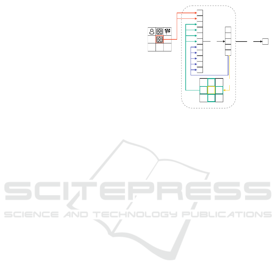
The cell network is a small recurrent network that

uses two fully connected layers as displayed in Fig-

ure 1. It takes a vector on the input which contains

information about the tile (red arrows), its neighbors

(green arrows) and values of the hidden states from

the last iteration (blue arrows). The ﬁrst fully con-

nected layer (FC-1) takes the input vector of size v

and computes h hidden states. The second fully con-

nected layer (FC-2) takes the h hidden states and cre-

ates one value which represents heuristic value for the

given grid tile. In case of the maze problem, the num-

ber estimates how many steps the agent has to take in

order to ﬁnd a goal in the maze if he starts at the given

tile.

As we mentioned, the cell network is recurrent so

the hidden states are a part of the input vector every

following iteration. In every iteration, each cell net-

work generates an output value using FC-2 (yellow

arrow) which is then being fed into the neighboring

cell networks in the next iteration (green arrows). All

the cell networks run for the same number of itera-

tions.

At the end of the last iteration, all cell networks re-

turn the ﬁnal heuristic value for their cell. That leaves

us with a matrix that contains a value for each tile of

the input grid. These values represent the heuristic

estimates for all the initial positions in the grid.

3.2 Training CSRN

In (Werbos and Pang, 1996), the authors showed that

training such structure using Stochastic Gradient De-

scent (SGD) methods does not converge efﬁciently.

We propose to use Bayesian Optimization (BO), as

it is a universal approach, which does not require

any additional assumptions on the objective function.

E.g., for mentioned SGD, this function has to be dif-

ferentiable, which heuristic functions are not in gen-

eral. To train the CSRN, we use BO with Gaussian

processes to optimize the objective function.

Input maze image

FC-2

Iteration outputs

Recurrent cell

Heuristic value

FC-1

FC-2

Figure 1: Cell network architecture. FC-1 represents a fully

connected layer which takes v inputs and returns h outputs;

FC-2 represents a fully connected layer which takes h in-

puts and returns one value; red arrows - ﬁxed grid tile en-

coding; green arrows - neighbor values from previous iter-

ation; blue arrows - feeding hidden states to next iteration;

yellow arrow - computation of intermediate result for one

iteration using FC-2.

3.3 Architecture Parameters

There are parameters of the cell network, but also for

the CSRN structure as a whole.

The cell network, as described in (Ilin et al.,

2008), requires number of recurrent iterations and

number of hidden states as parameters.

The number of iterations inﬂuences how much of

the actual search the cell network simulates during its

run but it does not inﬂuence the number of trainable

weights. It does, however, inﬂuence the run time of

the network.

On the other hand, the number of the hidden states

directly inﬂuences the number of trainable weights in

the whole architecture.

Let us say that the input vector v consists of n val-

ues which describe the grid tile, m values which con-

tain values of all tile’s neighbors and h values which

are the hidden state values from the previous iteration.

The total number of trainable weights w in such net-

work is then computed as

w = (n + m + h) ∗ h +h (1)

The CSRN can be used for any size of the input

grid, therefore it is a scale-free architecture. For all

our domains in this work, we parametrize the local-

ity of the cells as a 4-neighborhood, as we only as-

sume that the state can change by moving one cell up,

down, left and right (intuitively representing a robot

or agent on the grid). However, it is possible to deﬁne

the neighborhood in a different manner depending on

Learning Heuristic Estimates for Planning in Grid Domains by Cellular Simultaneous Recurrent Networks

205

...

}

grid tile encoding

neighbors' values

hidden states

Figure 2: General input vector encoding. First n values rep-

resent the grid tile encoding. Next m values are iteration

outputs from neighboring tiles. The last h values are hidden

states computed in the last iteration.

the actions available in the domain we are solving.

Deeper analysis of the action structure and its mani-

festation in the locality parametrization of the CSRNs

is left for future work.

4 PROBLEM DOMAINS

As we already mentioned, (Ilin et al., 2008) uses maze

traversal problem as the only domain which is also

used in (Urbanovsk

a et al., 2020). One property of the

maze domain is that the 2D grid representation con-

tains the whole state space of the problem. We can

create every state in the state space by simply mov-

ing the agent in the maze onto every free tile on the

grid. That led us to believe that the CSRNs’ success

may be caused simply by this property of the maze

domain, which is in core a simple problem from the

planning perspective. Intuitively, the only process the

CSRN has to learn is iterative gradient propagation

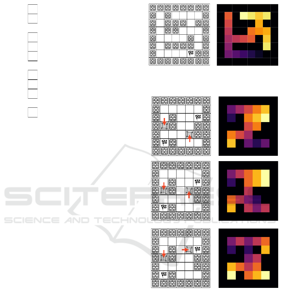
through the maze as shown in Figure 3. That creates

an optimal heuristic for such problem, provided that

the already ﬁlled cells are not overwritten.

Therefore, we decided to test out the CSRN ar-

chitecture on Sokoban domain, which is one of the

hardest classical planning problems (it falls into the

PSPACE-complete class). It can be easily represented

by a grid which makes it a perfect candidate for the

CSRN architecture, but its whole state space certainly

cannot be represented by one-dimensional 2D grid.

8.0

14.0 13.0 12.0 13.0

7.0

11.0

6.0 9.0

10.0 11.0

5.0 6.0 7.0 8.0

12.0

4.0

13.0

3.0 2.0 1.0 0.0

Figure 3: Gradient propagated through an example maze

instance. The goal tile should be equal to 0, each tile next

to it 1 and so on.

1.0 2.0 1.0 2.0 3.0

0.0 0.0 4.0

1.0 2.0

4.0 3.0 2.0 3.0

5.0 3.0 4.0 5.0

1.0 2.0 3.0 4.0 5.0

0.0 3.0 4.0 5.0

2.0

3.0 2.0 1.0 0.0

4.0 2.0 1.0 2.0

1.0 2.0 3.0 4.0 5.0

0.0 4.0 5.0 6.0

3.0 4.0

4.0 3.0 2.0

5.0 1.0 0.0 1.0

Figure 4: Gradient propagated through an example Sokoban

instance in 3 steps. The desired actions are for each map

conﬁguration are displayed as red arrows. The gradient nav-

igates the agent to a tile where it can make a decision that

creates a new state that is closed to a goal state.

4.1 Input Encoding

The cell network takes a vector on the input, so its cor-

responding grid tile has to be processed accordingly.

In Figure 2, we can see the general input vector struc-

ture for the cell network which is very similar for both

maze and Sokoban domain.

First n values of the vector describe the objects

present at the given grid tile. In case of maze it is rep-

ICAART 2022 - 14th International Conference on Agents and Artiﬁcial Intelligence

206

resented by 2 binary values, one for a goal and one for

a wall. In case of Sokoban there is one more binary

value that represents the presence of a box. These val-

ues stay the same in every recurrent iteration of the

cell network.

Next m values are output values from m neighbor-

ing grid tiles. In both domains we have only 4 possi-

ble actions which represent 4 possible movements on

the grid, so 4 values in total. Each problem instance

is surrounded by walls so the agent cannot step out

of the world, therefore we can wrap the neighborhood

around and not break any rules of the domain. That

is crucial because we need every cell network to have

input of the same size. The neighbor values change

in every iteration based on the previous results of the

neighboring cells.

Last h values are values of the hidden states. Their

number is set by a selected parameter. These values

change every iteration and at the start they are initi-

ated to −1.

4.2 CSRN Output

As described in Section 1, each cell network returns

one value at the very end of the CSRN computation.

In this section, we focus on the output as a whole

where we work with all the values returned by all the

cell networks.

Each grid tile is evaluated by a cell network, so

we can create an output grid with all the generated

values that has the same size as the input grid which

represents the problem as shown in Figure 3.

As we already stated, complete state-space of a

maze can be represented by the grid per se and we can

clearly see how to interpret the output of the CSRN in

this domain. Each cell in the output grid corresponds

to a heuristic value for a state where agent stands on

the given tile.

That is a great advantage for such simple domain

as the maze domain because we can run the CSRN

once and get heuristic values for the whole state-space

at the same time. That means that the heuristic com-

putation does not have to be repeated through the rest

of the search algorithm which can greatly contribute

to the algorithm’s performance. Sadly this only holds

for domains, where we can represent the whole state-

space by the output grid.

Sokoban is a more complex domain and its state-

space is much bigger and depends on different ele-

ments than just the position of the agent. Because of

the boxes that are present, the problem becomes ex-

ponential and to create one output with all heuristic

values we would have to create exponentially many

grids with all box combinations to be able to evaluate

the CSRN only once.

Creating a multi-dimensional output of the CSRN

is certainly an interesting direction for future re-

search, but in this work we decided to use 2D projec-

tion of the problem to be able to interpret the output

grid. The downside of this approach is that it is nec-

essary to evaluate the CSRN every time a box moves.

That is still less heuristic function calls than many

heuristics use because it is very common to evaluate

the heuristic function for every encountered state.

Thanks to this approach, we can then create a 2D

output grid which contains heuristic values for all the

agent positions in the world with particular box con-

ﬁguration. Therefore it is basically a projection over

two variables (x, y) that describe agent’s position. We

could do the same for any two variables and create a

2D representation which can be used as a source of

heuristic values for a subset of states. However, using

agent’s position seemed the most intuitive in this case.

Selection of the variable which are suitable for

such projection is a direction of research of itself

and it is not a problem, we will further discuss in

this work. However, with good selection strate-

gies, it would be possible to create such projection

for arbitrary problem and therefore create a domain-

independent framework that uses graphical represen-

tation on a grid.

5 CSRN TRAINING

Training of the CSRN architecture is a well-known

bottleneck of the approach as stated in (Werbos and

Pang, 1996). There have been many approaches to

training the architecture, but overall the training can

be very slow especially on a large number of samples.

We use a very small number of training samples of

small sizes because in this work we mainly focus on

generalizing and scaling abilities of the CSRN archi-

tecture.

Due to these reasons, we decided to use BO with

5 steps and 3 restarts which runs for 5000 iterations.

The objective function we want to optimize counts

number of incorrect decisions the network would

make in search using the learned heuristic. It is a

function analogous to function used in (Ilin et al.,

2008), thus the optimization algorithm aims to de-

crease the number of incorrect decisions made based

on the learned heuristic values. Incorrect decision is

such decision that is not present in any solution for

the problem.

Learning Heuristic Estimates for Planning in Grid Domains by Cellular Simultaneous Recurrent Networks

207

5.1 Objective Function

Before training the network, we have to create a struc-

ture that contains all ”correct decisions”. To do so, we

generate the whole state-space for the given instance

and ﬁnd all solutions for every existing state. Such

exhaustive search is costly, therefore, we only train

the network on smaller number of problem instances

that can be solved exhaustively in a reasonable time.

Once we have all plans for all possible states in

the state-space, we go through all the plans and mark

every decision that occurs in the plans. We know for

sure that every one of these decisions leads to a goal

state, because it is a part of a solution to the problem.

That way, we are able to train the network not only

on a subset of solutions but on all the existing solu-

tions which hopefully provides us with more general

knowledge about the problem domain.

In case of the maze domain, the exhaustive evalu-

ation does not create a problem, as we can run a basic

search algorithms from the goal and go through every

tile in the maze which guarantees that we ﬁnd all the

possible plans.

Exhaustive evaluation for one Sokoban map is a

very costly procedure. Therefore, we had to train the

network only on very small samples we were able to

exhaustively evaluate in a reasonable amount of time.

One evaluation requires creating states for all possible

box and agent position combinations and looking for

all solutions in every created state.

It might seem that the evaluation function and cre-

ating all possible plans is rather a tedious approach.

There are examples in the literature which use only

optimal plans for training (Shen et al., 2020). Our

reasoning behind training on all existing plans is that

the network might be able to make more informed de-

cisions in problematic parts of the state-space where

other heuristics struggle or where the optimal solution

may never lead to. We also hope it is going to prevent

reaching dead-ends

which is a great problem specif-

ically in the Sokoban domain. This approach prevents

expanding the dead-end states, however, its behaviour

in the dead-end is not being learned.

5.2 Parameter Selection

As stated in Section 3.3, there are several parameters

in the CSRN architecture that have to be set. For the

number of recurrent iterations and number of hid-

den states we trained architectures with different pa-

A dead-end state in planning is a state from which

no goal state is reachable. An example of a dead-end in

Sokoban is a state, where a box is in a corner, which is not

a goal.

rameter combinations. In the (Ilin et al., 2008), the

authors used 20 recurrent iterations and 15 hidden

states for the network. However, that was for the maze

domain. That is unfortunately not much information

on how to modify the values in order to process the

Sokoban domain. Therefore, we trained multiple dif-

ferently parametrized architectures and based on their

performance we used the most successful one in the

planning experiments.

Another mentioned parametrization of the archi-

tecture is based on the neighborhood deﬁnition. In

this case, in both the maze and Sokoban domains we

have one agent which is allowed to move by one tile

in its 4-neighborhood. Therefore the neighborhood

function can be reused for both domains.

5.3 CSRN Convergence

Since we are using BO to train the network we wanted

to demonstrate how the network converges on one

maze sample. We are testing convergence of the ob-

jective function, thus we want the number of incorrect

decisions made by the trained network equal to zero.

The training was deployed 400 times with the limit of

1000 iterations and the results can be seen in Figure 5.

We have observed that the success of the optimization

heavily relies on the initial weights which are sampled

randomly from given intervals.

In Figure 5 we see how the objective function con-

verges to zero during the training. The lowest num-

ber of iterations is 0 which means that the initial it-

eration was good enough to ﬁnd weights that yielded

no wrong decisions. On the other hand, we see that

the number of iterations can lead to hundreds. Even

though the correct gradient propagation in only one

maze instance is a very simple task, the initialization

plays a great part in the speed of training. Lucky ini-

tialization can lead to almost immediate success while

a bad initialization can lead to great prolonging. Some

of the runs did not even ﬁnish with no mistakes in the

given 1000 iterations.

6 EXPERIMENTS

We want to look at multiple properties of the trained

CSRN and decide whether it is a suitable approach for

neural heuristic learning for graphically represented

problems.

First, we want to take the trained architectures and

see their generalizing capabilities on different unseen

problem instances. That will show us if training on a

small number of samples provides the network with

ICAART 2022 - 14th International Conference on Agents and Artiﬁcial Intelligence

208

Figure 5: Convergence graph for training CSRN on one

maze instance 400 times for the ﬁrst 200 iterations. Blue

line represents average number of wrong decisions per

training iteration. The grey band represents standard de-

viation.

a knowledge base that can be reused on different but

similar problems.

Next, we want to see how the CSRN scales-up

with the learned knowledge. In case of the maze do-

main, we use it on larger instances and in case of

the Sokoban, we create larger instances and instances

with more boxes which can both increase the com-

plexity of the problem.

The last experiments regard the planning perfor-

mance which is also an important aspect of our work.

We integrated the CSRN as a heuristic function into

our classical planning solver and we want to compare

the performance of CSRN in comparison with other

heuristic functions on the same data sets.

All codes used for the experiments were imple-

mented in Julia, including the domain-speciﬁc plan-

ners which use naive implementation of heuristics

described in Section 2.2. That way, we have a fair

comparison in terms of the evaluation.

Due to the nature of our data we have imple-

mented domain-speciﬁc planners in Julia together

with all the mentioned heuristic functions. All exper-

iments were performed on the same machine with 64

CPU cores, 346 GB of memory and a GPU for com-

putation of the neural networks required in the plan-

ning process.

To evaluate the results we use the same metrics

for all the experiments. First we look at average path

length denoted as ”avg pl” which shows average so-

lution length over the given data set. Next is the aver-

age number of expanded states denoted as ”avg ex”

which shows average number of expanded states dur-

ing the search. And last is the coverage denoted as

”cvg” which shows solving success rate.

Experimental codes were based on

https://github.com/urbanm30/nn-planning.

6.1 Generalization and Scaling

Experiments

In Section 5.2 we mentioned that we had to train

multiple networks with different parameter conﬁgu-

rations. We then integrated trained network in a plan-

ner and used them to solve different unseen data sets.

Each data set in this branch of experiments contains 5

unseen problem instances. For each data set we also

provided reference solution that has been achieved by

using GBFS and the blind heuristic which is denoted

as ”ref” in Table 1 and Table 2. In both tables, each

CSRN conﬁguratoin is encoded as ”number of recur-

rent iterations”−”number of hidden states”.

CSRNs for the maze domain were trained on 5

problem instances of size 5x5. The parameters were

selected from following

• number of recurrent iterations = [10, 20]

• number of hidden states = [5, 10 ,15].

We then evaluated the trained networks on data set

5x5 which contains 5 unseen samples of size 5x5 and

on data set 10x10 which contains 5 unseen samples of

size 10x10.

CSRNs for the Sokoban domain were trained on

1 problem instance of size 3x3 with one box. The

parameters were selected from following

• number of recurrent iterations = [10, 20, 30]

• number of hidden states = [15, 30].

Sokoban is a more complicated domain in terms of

difﬁculty so we decided to scale-up both the size and

the number of boxes. Each mentioned data set con-

tains 5 unseen problem instances. First we have 2

data sets of size 3x3 with one and two boxes. Then

we have 3 data sets with samples of size 6x6 with

one, two and three boxes.

The search for the generalizing and scaling exper-

iments was limited by number of expanded states for

each sample which was set to 2x the reference solu-

tion.

6.1.1 Maze Domain

In Table 1 we can see results for all mentioned data

sets and CSRN conﬁgurations. All conﬁgurations

solved all problems in both data sets with the best pos-

sible solution lengths. The only difference is in the

number of expanded states. All CSRN conﬁgurations

managed to expand less states than the reference so-

lution in both data sets. The conﬁguratoins with best

results are the 20-15 which achieved lowest number

of expanded states on the 5x5 data set and the 10-10

conﬁgurations which achieved the lowers number of

Learning Heuristic Estimates for Planning in Grid Domains by Cellular Simultaneous Recurrent Networks

209

expanded states one the 10x10 data set. These two

conﬁgurations are further used in the planning exper-

iments.

6.1.2 Sokoban Domain

In Table 2 we see results for all the CSRN conﬁgu-

rations trained for Sokoban. The ﬁrst two data sets

which both have samples of size 3x3 were not a prob-

lem in terms of coverage because all CSRNs were

able to solve all the problems. The ﬁrst unsolved in-

stances appeared in the 6x6 data set with one box.

Conﬁguration with the highest coverage (most

solved problems) is clearly 10-30 which did not solve

only one problem and also has lower number of ex-

panded states on 4/5 data sets.

From the solution length perspective, no CSRN

was able to produce shorter solutions than the refer-

ence solver. Four conﬁgurations were able to ﬁnd the

same average solution length for 2 data sets. From

these four conﬁgurations we selected the 30-30 be-

cause it has the highest coverage and also expanded

less states than the reference point in 3/5 data sets

compared to the other 3 conﬁgurations.

Based on the results, conﬁgurations 10-30 and 30-

30 are further used in the planning experiments.

6.2 Planning Experiments

Each data set for the planning experiments contains

50 samples which are all unseen for the trained CSRN

architectures. Each problem instance in the planning

experiments is limited by a time limit of 10 minutes.

For each domain, we used two trained networks that

were evaluated as the best ones. In case of maze, we

use CSRN conﬁgurations 10-10 and 20-15 which are

denoted as CSRN-1 and CSRN-2. In case of Sokoban,

we use CSRN conﬁgurations 10-30 and 30-30 which

are placed in the same row in Table 3 as CSRN-1 and

CSRN-2.

We can see all the results in Table 3. First four

columns contain planning experiments where we used

four data sets of different sized mazes - 8x8, 16x16,

32x32, 64x64. Last three columns in Table 3 con-

tains three data sets of Sokoban data - 8x8, 10x10

- Boxoban, 16x16. The data used in 10x10 data set

were sampled from the original Boxoban (Guez et al.,

2018) data set.

The CSRNs were successful in the maze domain

in terms of coverage because they were able to solve

every problem instance in all four data sets. In terms

of solution length, they also found optimal solutions

for 3/4 data sets. A drawback we can see in the CSRN

performance is the number of expanded states which

is greater than even the simplest heuristic. That means

that the heuristic generated by CSRN was often mis-

leading for the search and caused selection of wrong

states in the algorithm. However, since the heuris-

tic is precomputed once for the whole maze (see Sec-

tion 4.2), the ﬁnal efﬁciency of the search does not lag

behind the classical methods.

The Sokoban domain is a lot more complex and

size of the instances in the planning experiments is

higher than in the generalizing and scaling experi-

ments. In the 8x8 data set, we can see that both CSRN

conﬁgurations were able to achieve 0.98 coverage and

expand nearly half the states compared to the blind

heuristic. The performance gets worse in the 16x16

data set where CSRNs cannot solve any of the given

instances. In the 10x10 - Boxoban data set we can see

that the CSRNs solved at least some of the instances

but the coverage is very low.

We also want to address the low coverage of the

LM-cut and h

heuristics which is caused by the

complexity of the domain as well as the computa-

tional time they require. We can see that CSRN has an

advantage over these two heuristics especially in the

8x8 data set. As we stated in Section 4.2, CSRN has

to be evaluated only once for a new box conﬁguration

so the evaluation is not running for every new state

and its outputs can be saved and reused. That seems

to be a great advantage in the Sokoban domain. While

using the CSRN we can expand more states quicker

because when we compute heuristic (run the CSRN)

it provides heuristic values for a whole subset of states

instead of just one state.

6.3 Discussion

Results presented in 6.1 and 6.2 show us that the

CSRN architecture is able to scale-up for both given

domains. In case of the maze domain, we see impres-

sive performance for all presented data sets and the

planning experiments. This result is to be expected

due to the domain’s complexity.

Much more interesting are the Sokoban results

where we see CSRN’s ability to generalize over in-

comparably more difﬁcult problem instances. Con-

sidering the fact that the CSRN was trained on empty

3x3 maze with one box its performance on 6x6 and

8x8 instances is very impressive. More importantly, it

was fully able to adapt to problems with higher num-

ber of boxes. Adding boxes to the Sokoban prob-

lem presents a large number of complications for

the heuristic. There are overlapping trajectories, ex-

tended movement rules as only one box can be pushed

at a time and other aspects which make the problem

more complex.

ICAART 2022 - 14th International Conference on Agents and Artiﬁcial Intelligence

210

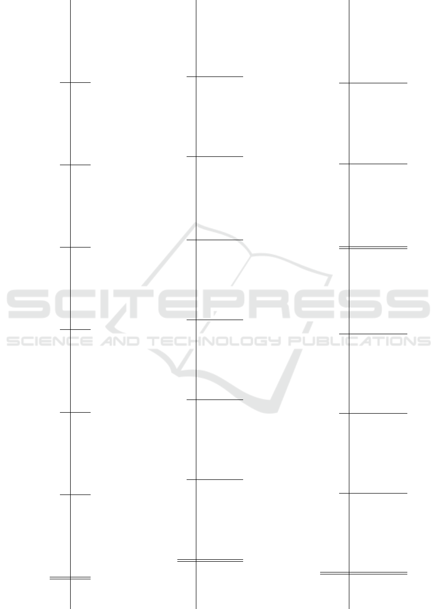
Table 1: CSRN evaluation performed on maze domain. Reference solver is GBFS with blind heuristic. Each CSRN conﬁguration is named by its number of reccurent iterations

and number of hidden states connected with a dash. Best results are written in bold lettering.

ref 10-5 10-10 10-15 20-5 20-10 20-15

avg pl avg ex cvg avg pl avg ex cvg avg pl avg ex cvg avg pl avg ex cvg avg pl avg ex cvg avg pl avg ex cvg avg pl avg ex cvg

5x5 5.6 19.2 1 5.6 12.6 1 5.6 12.8 1 5.6 11.4 1 5.6 10.8 1 5.6 13.6 1 5.6 10.0 1

10x10 11.2 80.8 1 11.2 48.8 1 11.2 33.6 1 11.2 46.0 1 11.2 51.0 1 11.2 42.6 1 11.2 40.6 1

Table 2: CSRN evaluation performed on Sokoban domain. Reference solver is GBFS with blind heuristic. Each CSRN conﬁguration is named by its number of reccurent

iterations and number of hidden states connected with a dash. Best results are written in bold lettering.

ref 10-15 10-30 20-15 20-30 30-15 30-30

size boxes avg pl avg ex cvg avg pl avg ex cvg avg pl avg ex cvg avg pl avg ex cvg avg pl avg ex cvg avg pl avg ex cvg avg pl avg ex cvg

3x3 1 6.0 23.6 1 6.0 22.4 1 6.4 21.6 1 6.0 28.4 1 6.0 23.8 1 6.0 22.8 1 6.0 29.6 1

3x3 2 5.2 10.8 1 5.4 18.4 1 5.4 18.4 1 5.2 20.0 1 5.2 19.6 1 5.2 20.0 1 5.4 7.6 1

6x6 1 21.0 340.8 1 29.8 469.8 1 29.0 261.8 1 26.2 454.2 1 26.25 430.75 0.8 27.0 465.2 1 27.25 466.5 0.8

6x6 2 21.8 1210.6 1 39.5 950.5 0.4 49.25 997.5 0.8 39.5 951.5 0.4 40.75 1496.75 0.8 29.5 946.0 0.4 33.25 658.5 0.8

6x6 3 28.6 12421.0 1 54.0 18217.5 0.4 72.8 10731.0 1 57.8 11195.8 1 79.0 13134.25 0.8 51.5 17838.0 0.4 50.2 8471.2 1

Table 3: Planning experiments for both maze and Sokoban domains.

Maze Sokoban

8x8 16x16 32x32 64x64 8x8 10x10 - Boxoban 16x16

avg pl avg ex cvg avg pl avg ex cvg avg pl avg ex cvg avg pl avg ex cvg avg pl avg ex cvg avg pl avg ex cvg avg pl avg ex cvg

blind 11.64 27.42 1 23.36 96.82 1 46.2 267.28 1 104.72 1085.66 1 111.24 3.5k 1 1.2k 66k 1 30k 52k 0.54

ED 10.76 14.58 1 23.36 48.14 1 46.2 129.7 1 104.72 561.44 1 31.10 0.5k 1 45.64 8.2k 1 115.33 12.6k 0.54

10.76 10.76 1 23.36 23.36 1 46.2 46.2 1 104.72 104.72 1 - - 0.04 - - 0 - - 0

LM-cut 10.76 10.76 1 23.36 23.36 1 - - 0 - - 0 - - 0 - - 0 - - 0

CSRN-1 10.88 28.98 1 23.36 105.6 1 46.2 357.5 1 104.72 1572.68 1 41.65 1.7k 0.98 37.67 2.1k 0.06 - - 0

CSRN-2 10.88 26.9 1 23.36 105.02 1 46.2 356.44 1 104.72 1607.86 1 47.76 2.1k 0.98 36.0 968.0 0.04 - - 0

Learning Heuristic Estimates for Planning in Grid Domains by Cellular Simultaneous Recurrent Networks

211

Based on the results we can report that the CSRN

is capable of generalizing and scaling not only in the

maze domain which we consider a simple baseline but

also in the Sokoban domain.

7 CONCLUSION

We successfully trained CSNR architecture on both

maze and Sokoban domains and evaluated its scal-

ing and generalizing ability on unseen problem in-

stances. We also integrated trained CSRNs into a

planner and compared their performance with other

commonly used heuristic functions. As we already

stated, we are using the image-like grid representa-

tion of the problems. Thanks to that, we can say that

we work with a model-free planning framework be-

cause our planner does not require a domain / problem

model for the computation.

The generalizing and scaling experiments showed

that the CSRN architecture is able to generalize very

well on maze domain where it outperformed the refer-

ence solution in all data sets. In case of the Sokoban

domain, we were able to achieve 96% coverage and

even though the CSRN was ﬁnding longer solution in

general, it was also able to decrease number of ex-

panded states compared to the reference solution.

The planning experiments showed that the CSRN

for maze domain provided comparable results to the

classical heuristics, however, it expanded a larger

amount of states in the process. In the Sokoban do-

main, we saw a great coverage on the 8x8 data set

which contained larger instances than the data sets in

generalizing and scaling experiments. However, we

also saw limitations of the trained conﬁgurations as

the results on the other two data sets showed next to

no coverage. That is caused by the size of the prob-

lem instances which inﬂuence the complexity as well.

Still, training the network on one 3x3 sample pro-

vided us with great results on the 8x8 data set and

a promising direction for a follow-up research of the

CSRN ability to generalize.

These results show us that the CSRN architec-

ture might be the right tool for grid-based domains in

terms of heuristic computation. Other further research

direction would be to explore achieving domain-

independence of this approach. So far, we have two

ways of achieving that. One is creating an algorithm

that would select appropriate variables in the problem

domain which would allow us to create a 2D projec-

tion of the problem. The other way is creating an al-

ternative representation of the problem which would

be still processed by the CSRN architecture but with-

out the condition of the grid structure, similarly as

in Natural Language Processing using a linear vector

representation, for instance.

Addressing these ideas could lead to a model-free,

scale-free and domain-independent heuristic function

learned by a neural network on small tractable prob-

lem samples. In the future, we would like to focus on

these mentioned challenges and provide such frame-

work that could process any given problem.

ACKNOWLEDGEMENTS

The work of Michaela Urbanovsk

a was

supported by the OP VVV funded project

CZ.02.1.01/0.0/0.0/16019/0000765 “Research

Center for Informatics” and the work of Anton

ın

Komenda was supported by the Czech Science

Foundation (grant no. 21-33041J).

REFERENCES

Aeronautiques, C., Howe, A., Knoblock, C., McDermott,

I. D., Ram, A., Veloso, M., Weld, D., SRI, D. W., Bar-

rett, A., Christianson, D., et al. (1998). Pddl— the

planning domain deﬁnition language. Technical re-

port, Technical Report.

Asai, M. and Fukunaga, A. (2017). Classical planning in

deep latent space: From unlabeled images to PDDL

(and back). In Besold, T. R., d’Avila Garcez, A. S.,

and Noble, I., editors, Proceedings of the Twelfth In-

ternational Workshop on Neural-Symbolic Learning

and Reasoning, NeSy 2017, London, UK, July 17-18,

2017, volume 2003 of CEUR Workshop Proceedings.

CEUR-WS.org.

Asai, M. and Fukunaga, A. (2018). Classical planning in

deep latent space: Bridging the subsymbolic-symbolic

boundary. In Thirty-Second AAAI Conference on Ar-

tiﬁcial Intelligence.

Bundy, A. and Wallen, L. (1984). Breadth-ﬁrst search. In

Catalogue of artiﬁcial intelligence tools, pages 13–13.

Springer.

Groshev, E., Tamar, A., Goldstein, M., Srivastava, S., and

Abbeel, P. (2018). Learning generalized reactive poli-

cies using deep neural networks. In 2018 AAAI Spring

Symposium Series.

Guez, A., Mirza, M., Gregor, K., Kabra, R., Racaniere,

S., Weber, T., Raposo, D., Santoro, A., Orseau,

L., Eccles, T., Wayne, G., Silver, D., Lilli-

crap, T., and Valdes, V. (2018). An investi-

gation of model-free planning: boxoban levels.

https://github.com/deepmind/boxoban-levels/.

Hoffmann, J. (2001). Ff: The fast-forward planning system.

AI magazine, 22(3):57–57.

Ilin, R., Kozma, R., and Werbos, P. J. (2006). Cellular srn

trained by extended kalman ﬁlter shows promise for

ICAART 2022 - 14th International Conference on Agents and Artiﬁcial Intelligence

212

adp. In The 2006 IEEE International Joint Confer-

ence on Neural Network Proceedings, pages 506–510.

IEEE.

Ilin, R., Kozma, R., and Werbos, P. J. (2008). Beyond feed-

forward models trained by backpropagation: A prac-

tical training tool for a more efﬁcient universal ap-

proximator. IEEE Transactions on Neural Networks,

19(6):929–937.

Pommerening, F. and Helmert, M. (2013). Incremental lm-

cut. In Twenty-Third International Conference on Au-

tomated Planning and Scheduling.

Richter, S. and Westphal, M. (2010). The lama planner:

Guiding cost-based anytime planning with landmarks.

Journal of Artiﬁcial Intelligence Research, 39:127–

177.

Shen, W., Trevizan, F., and Thi

ebaux, S. (2020). Learning

domain-independent planning heuristics with hyper-

graph networks. In Proceedings of the International

Conference on Automated Planning and Scheduling,

volume 30, pages 574–584.

Torralba, A., Alcazar, V., Borrajo, D., Kissmann, P., and

Edelkamp, S. (2014). Symba: A symbolic bidirec-

tional a planner. International Planning Competition,

pages 105–109. cited By 27.

Urbanovsk

a, M., B

ım, J., Chrestien, L., Komenda, A., and

Pevn

y, T. (2020). Model-free automated planning us-

ing neural networks. In Proceedings of the 1st Work-

shop on Bridging the Gap Between AI Planning and

Reinforcement Learning (PRL) of the International

Conference on Automated Planning and Scheduling,

pages 7–15.

Werbos, P. J. and Pang, X. (1996). Generalized maze navi-

gation: Srn critics solve what feedforward or hebbian

nets cannot. In 1996 IEEE International Conference

on Systems, Man and Cybernetics. Information Intelli-

gence and Systems (Cat. No. 96CH35929), volume 3,

pages 1764–1769. IEEE.

White, W. E., Iftekharuddin, K. M., and Bouzerdoum, A.

(2010). Improved learning in grid-to-grid neural net-

work via clustering. In International Joint Conference

on Neural Networks, IJCNN 2010, Barcelona, Spain,

18-23 July, 2010, pages 1–7. IEEE.

Learning Heuristic Estimates for Planning in Grid Domains by Cellular Simultaneous Recurrent Networks

213