Incremental Feature Learning for Fraud Data Stream

Armin Sadreddin and Samira Sadaoui

Department of Computer Science, University of Regina, Regina, Canada

Keywords:

Incremental Feature Learning, Transfer Learning, Data Stream, Data Privacy, Credit-card Fraud Data.

Abstract:

Our research addresses the actual behavior of the credit-card fraud detection environment where ﬁnancial

transactions containing sensitive data must not be amassed in a considerable amount to train robust classiﬁers.

We introduce an adaptive learning approach that adjusts frequently and efﬁciently to new transaction chunks;

each chunk is discarded after each training step. Our approach combines transfer learning and incremental

feature learning. The former improves the feature relevancy for subsequent chunks, and the latter increases

performance during training by dynamically determining the optimal network architecture for each new chunk.

We show the effectiveness and efﬁciency of our approach experimentally on an actual fraud dataset.

1 INTRODUCTION

A tremendous volume of credit card transactions is

conducted daily, especially with COVID-19. Nev-

ertheless, this e-commerce activity attracted many

fraudsters and led to monetary losses for credit card

holders. For instance, for 2019, the Nelson Report es-

timated the worldwide ﬁnancial loss from Credit Card

Fraud (CCF) to $28.65 billion (Worldwide Credit

Card Fraud Statistics 2019, 2020). Over the last ten

years, users that revealed at least one CCF soared

by 71% in Canada (Credit Card Fraud Statistics In

Canada 2021, 2021). Detecting fraudulent payments

necessities vital resources, such as powerful process-

ing, ample data storage, and human expertise. CCF

detection is complex to address due to the follow-

ing challenges: (1) Transactions are generated con-

tinuously and speedily. In this data stream context,

fraud must be detected in real-time to avoid losses

on the users’ side; (2) Conventional Machine Learn-

ing Algorithms (MLAs), including deep learning, re-

quire storing many transactions to conduct training.

However, ﬁnancial data must not be accumulated in a

large quantity by the learned models because of data

sensitivity and conﬁdentiality; and (3) MLAs can-

not adapt previous knowledge to newly available data

to improve their accuracy, making the fraud detec-

tion models obsolete and unreliable in the long run.

Most of the studies on CCF detection employed con-

ventional MLAs (non adaptive) that are inadequate

for the CCF learning environment. Additionally, in

the industry, a new fraud prediction system is created

from scratch for every number of days to learn the

new behavior from incoming transactions (Lebichot

et al., 2020). However, re-training for each new data

is time-consuming, and the past learned knowledge is

lost.

To overcome the above challenges, we develop

a new adaptive learning algorithm that adjusts fre-

quently and efﬁciently to new transaction data,

grouped in chunks or mini-batches. We decide how

much data to collect in each chunk depending on the

incremental training frequency (i.e., every day or ev-

ery week). More the frequency is shorter, less sensi-

tive data is accumulated. In our study, a chunk con-

tains the payment transactions of one day, which is

still enough for a robust adaptation. We process one

chunk at a time in the short-term memory and discard

it after each model’s adaptation, without the necessity

of storing it. The proposed adaptive approach com-

bines transfer learning and incremental feature learn-

ing. Thanks to transfer learning, we extract more

valuable features from the original ones and reuse the

new features for the subsequent transaction chunks.

For instance, in the image processing area, the ﬁrst

layers of the neural network extract more representa-

tive features that can be reused in another image pro-

cessing task. Following the same reasoning, we use

the ﬁrst layers to collect more beneﬁcial features and

then add a new network to utilize those features. By

doing so, we take advantage of the previous chunks’

knowledge.

Our Incremental Feature Learning (IFL) algo-

rithm adapts gradually to the new transaction chunks

268

Sadreddin, A. and Sadaoui, S.

Incremental Feature Learning for Fraud Data Stream.

DOI: 10.5220/0010812700003116

In Proceedings of the 14th International Conference on Agents and Artiﬁcial Intelligence (ICAART 2022) - Volume 3, pages 268-275

ISBN: 978-989-758-547-0; ISSN: 2184-433X

by (1) preserving the previously learned knowledge

and (2) dynamically adjusting the network architec-

ture for each new chunk to achieve the highest per-

formance during training. IFL expands the network

topology by adding new hidden layers and new units

during each adaptation phase. Determining the most

suitable model’s architecture leading to the best per-

formance is a complex problem. Our IFL approach

adds hidden units one by one until the model does not

converge anymore. Nevertheless, as we are chang-

ing the network architecture to increase the perfor-

mance, we may over-ﬁt the resulted model. Hence,

we utilize a validation chunk during training to avoid

over-ﬁtting after each extension. More precisely, only

the weights of the new hidden units are updated each

time and the previous units are frozen to store the pre-

vious knowledge. Thus, less computational time is

needed to conduct learning for each new chunk. In

this way, our IFL approach will always outperform

other incremental learning approaches as the former

continuously adapts its architecture to reach optimal

accuracy. Most of the architecture of past incremen-

tal learning approaches is permanently ﬁxed (Anowar

and Sadaoui, 2021), and the accuracy may not im-

prove when new chunks are fed to the model. Imple-

menting the IFL algorithm is challenging, requiring a

deep investigation of the building blocks and libraries

of MLA toolkits, such as creating a new hidden unit,

adding a new connection, and freezing the weights of

a old connection (not to be re-optimized). Moreover,

using a real CCF dataset, we create training, testing,

and validation data chunks and handle the highly im-

balanced chunks. For a robust validation of our IFL

algorithm, we develop four fraud classiﬁers, trained

on different chunks, and then compare their predic-

tive performances on unseen data. The experimental

results show the efﬁciency of the proposed learning

approach.

The study (Guan and Li, 2001) was the ﬁrst one

to develop an IFL approach. This approach, which

is elementary, adopted a network topology that is not

common because the input layer is directly connected

to the output layer. During training, it freezes all the

weights connected to the output unit. Although freez-

ing these weights can speed up training, it will how-

ever reduce the model’s performance. Also, this pa-

per does not provide details on the algorithm design

and its implementation. Our paper presents all the

stages of our IFL algorithm that learns progressively

from newly available chunks. Through a concrete ex-

ample, based on constructive neural networks, we il-

lustrate step by step the sophisticated behavior of our

adaptive approach.

2 RELATED WORK

We review recent research on detecting CCF and

highlight its weaknesses. The majority of studies con-

ducted batch learning, such as (Hassan et al., 2020)

that explored deep learning, like BiLSTM and Bi-

GRU, and classical learning, such as Decision Tree,

Ada Boosting, Logistic Regression, Random For-

est, Voting and Naive Base. Since the fraud dataset

is highly imbalanced, the authors adopted random

under-sampling, over-sampling and SMOTE. The hy-

brid of over-sampling, BiLSTM and BiGRU lead to

the highest accuracy. Another work (Nguyen et al.,

2020) also assessed several MLAs, including LSTM,

2-D CNN, 1-D CNN, Random Forest, ANN and

SVM, using different data sampling methods on three

credit-card datasets. LSTM and 1-D CNN combined

with SMOTE returned the best results. We believe

LSTM can be a good option for incremental learn-

ing since this algorithm can remember past data and

therefore creates predictions using the current inputs

and past data, leading to a better response to the en-

vironmental changes. In both papers, LSTMs and the

other models were trained on very large datasets, re-

quiring storing sensitive information forever. Nev-

ertheless, since user transactions are available incre-

mentally, conventional MLAs are inappropriate for

streaming data. Our proposed method aims to address

the real CCF classiﬁcation context.

In (Anowar and Sadaoui, 2020), the authors ﬁrst

utilized SMOTE-ENN to handle a highly imbalanced

CCF dataset and then divided the dataset into multiple

training chunks to simulate incoming data. They pro-

posed an ANN-based incremental learning approach

that learns gradually from new chunks using an in-

cremental memory model. For adjusting the model

each time, the memory consists of one past chunk (so

that data are not forgotten immediately) and one re-

cent chunk (to conduct the model adaptation). The

authors demonstrated that incremental learning is su-

perior to static learning. However, using two chunks

every time can be expensive computationally. Also,

since the ANN topology is ﬁxed, the model cannot

adapt to signiﬁcant changes in the chunk patterns. In

our study, the ANN architecture is dynamic to build

an optimal fraud detection model. Instead of using

two chunks simultaneously, leading to storing more

data, we use only one chunk. With transfer learning,

we take advantage of the previous chunk without stor-

ing it.

In (Bayram et al., 2020), the authors introduced

a Gradient Boosting Trees (GBT) approach, which is

just an ensemble of decision trees, to minimize the

loss function gradually. The ensemble is updated for

Incremental Feature Learning for Fraud Data Stream

269

Table 1: Original and Re-Sampled Training and Testing

Chunks.

(a) Highly Imbalanced Chunks

Original Dataset

Fraud Normal

473 283253

Chunk 1: transactions of day1

Train Ratio Test Ratio

101352 1:532 43437 1:529

Chunk 2: transactions of day2

Train Ratio Test and Validation Ratio

97255 1:689 41682 1:694

(b) Re-balanced Chunks

Train Chunk1

Fraud Normal Total

33383 101162 134545

Test Chunk1

Fraud Normal Total

14307 43355 57662

Train Chunk2

Fraud Normal Total

32047 97114 129161

Test Chunk2

Fraud Normal Total

6867 20811 27678

Validation Chunk2

Fraud Normal Total

6867 20811 27678

each new group of transactions by appending a new

Decision Tree to create a more robust GBT model.

The authors developed three models: static GBT

(batch learning), re-trained GBT (re-training all the

transactions by including the investigated ones), and

incremental GBT (ensemble). All these methods ne-

cessitate storing a tremendous quantity of user trans-

actions. The authors divided the credit-card dataset

into several sub-datasets w.r.t time (month) and eval-

uated the three models for each month (four months

in total). Although the re-trained GBT (performed

with 1.6 million transactions) achieved the best per-

formance, it is 3000 times slower than the incremen-

tal approach. Since re-training is too time-consuming,

we aim to improve the accuracy and training time for

learning incrementally.

3 DATA CHUNK PREPARATION

We utilize a public, anonymized CCF dataset consist-

ing of 284807 users’ purchasing transactions that oc-

curred during two days in September 2013 (Credit

Card Fraud Detection, Anonymized credit card trans-

actions labeled as fraudulent or genuine, 2016). It is

worth mentioning that CCF datasets are lacking in the

literature due to data conﬁdentiality. The 2-class fraud

dataset possesses 29 predictive features obtained with

the feature extraction method PCA. However, the two

features Time and Amount as kept as is, because their

actual values are essential for training. Time rep-

resents the seconds passed between the current and

the ﬁrst transactions in the dataset. After examining

the dataset, only 0.172% (492) of the transactions is

fraudulent. We found duplicated fraud data (19) that

we eliminated. We are in the presence of a highly im-

balanced dataset where the count of legitimate data

is much higher than the count of fraudulent data. In

this case, classiﬁers will be biased towards the Nor-

mal class and will wrongly classify the Fraud class.

We split the fraud dataset into two chunks us-

ing the transaction’s time: the ﬁrst chunk is related

to the ﬁrst day and the second chunk to the second

day. We use the ﬁrst chunk to perform transfer learn-

ing and the second chunk IFL. In Table 1 (a), using

the stratiﬁed method, we divide the ﬁrst chunk into

70% training and 30% testing, and the second chunk

into 70% training, 15% validation and 15% testing.

As observed, the training chunks are highly imbal-

anced. Hence, we adopt the successful over-sampling

method SMOTE using the new class distribution ra-

tio of Normal instances to Fraud instances equals 1.3.

We over-sample the Fraud class to keep all of them as

they are rare events. For example, the training chunk2

has a highly imbalanced class ratio of 1:689 that we

re-balance with the new ratio of 1.3. Table 1 (b) ex-

poses the re-sampled training, validation and testing

chunks.

4 INCREMENTAL FEATURE

LEARNING

For our fraud classiﬁcation problem, we ﬁrst build the

initial model on the ﬁrst chunk and then utilize the

transformed features to train on the second chunk us-

ing the optimal number of hidden units. Instead of re-

training from scratch the entire model for each new

chunk, we only train the newly added units and freeze

all the previous layers. This strategy will signiﬁcantly

decrease the training time so that the classiﬁer identi-

ﬁes fraud activities much faster. The most difference

of incremental learning from conventional learning is

that the former does not assume the availability of suf-

ﬁcient training data, as data are available over time

(Guan and Li, 2001). So, based on these facts, im-

proving learning for each newly supplied chunk is an

excellent approach.

ICAART 2022 - 14th International Conference on Agents and Artiﬁcial Intelligence

270

Algorithm 1 conducts transfer learning and then

IFL. We ﬁrst build the initial network with four fully

connected layers, where the ﬁrst layer has the input

features, the ﬁrst hidden layer 500 units, the second

hidden layer ten units, and the output layer one unit

for the binary classiﬁcation. The study (Anowar and

Sadaoui, 2020), which validated an incremental learn-

ing approach with the same credit-card dataset, deter-

mined that 500 units as the best number for the ﬁrst

hidden layer. Hence, we train this ﬁrst network on the

ﬁrst chunk. Then, after removing the output unit, we

reﬁt the initial model using previous knowledge and

the second chunk. Now, the second hidden layer rep-

resents the transformed features (called tSubset) i.e.,

the new dimensional space more relevant to the target

class because it is obtained with previous knowledge.

Here, tSubset contains the values corresponding to the

transformed features. For example, assume we have

100,000 transactions in the second chunk. Using the

reﬁtted model, we convert each transaction of 29 val-

ues to ten new values. So, our transformed tSubset

will contain 100,000 new data with 10 new features.

With transfer learning (Weiss et al., 2016), our model

takes information from a previously learned task and

uses it to learn a related task. The model can extract

useful features from the input features, and instead of

learning this knowledge again, we use it via the past

network.

We actually extend the initial network with two

sub-networks; the ﬁrst sub-NN considers the high-

level features, and the second sub-NN the low-level

features. We leverage both of them to predict the out-

put more efﬁciently. Also, the study (Wang et al.,

2014) showed that creating sub-networks according

to the features’ relevancy can lead to a better out-

come. We add the second sub-NN to improve more

the model’s performance. A similar idea is used in

the incremental approach deﬁned in (Guan and Li,

2001) by connecting the original inputs directly to the

output unit with the same motivation. Another paper

(Wang et al., 2021) compared the performance results

of connecting the inputs to the output unit directly.

These are the reasons we use high-level features for

creating the ﬁrst sub-NN and then low-level features

for creating the second sub-NN. Thus, we can gradu-

ally improve the accuracy using newly available data

without forgetting the previous knowledge (stored in

the previous weights). Also, the training time will be

much lower as we only train the new chunk and one

unit only per epoch. Our approach can be used for any

number of chunks by appending a new hidden layer to

the ﬁrst sub-NN.

Algorithm 2, proposed in our past study (Sadred-

din and Sadaoui, 2021), shows how to extend a sub-

NN with new hidden units and connections. The

main challenge is determining the number of units

that should be added to attain the best training perfor-

mance. In transfer learning, we add a predetermined

number of layers and units to the previously trained

model. It can lead to fewer layers/units, but, the re-

sulting model will return poor predictions. On the

other hand, it can add unnecessary layers/units, which

only increases the learning time. Since the numbers

of layers and units are predetermined, all the units are

trained together and not one at a time like our pro-

posed method. So, the training time will be very time-

consuming. We determine the needed number of units

in our work by adding and training them one by one.

This approach is highly efﬁcient computationally.

Furthermore, instead of computing the gradient

descent for all the new units at once for each epoch,

which is time-consuming, we utilize the “patience”

parameter as the early stopping criterion. Based

on the convergence threshold, this parameter checks

whether the error is reducing or not in a certain num-

ber of epochs.

4.1 An Illustrative Example

Based on the CCF chunks, we illustrate the behavior

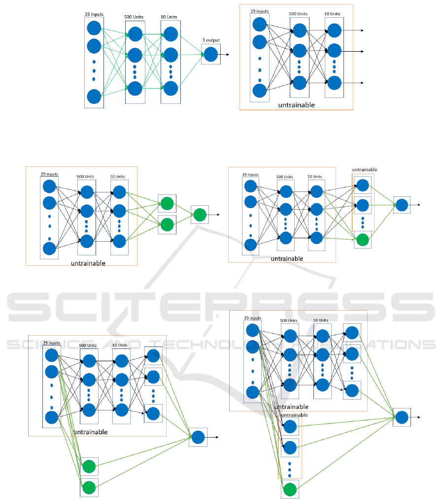
of our IFL algorithm in Figures 1, 2, and 3, where

the green color denotes new connections and new

units and the red color the frozen part of the NN

(weight are not re-learned). Figure 1 creates the ini-

tial NN and trains it on chunk1. After deleting the

output unit, the algorithm utilizes previously learned

weights and creates the reﬁtted model by training with

chunk2. Figure 2 ﬁrst adds the ﬁrst sub-NN to the ini-

tial model and then keeps training on the data of the

transformed features by including new hidden units

and connections and freezing past weights until the

training performance is not converging anymore. Fig-

ure 3 creates the second sub-NN using the original

features, connects it to the output unit of the previous

model, freezes all the previous weights, and trains it

on chunk2 until the model is not converging anymore.

5 VALIDATION

Since the CCF features have different value ranges

and with signiﬁcant discrepancies, we ﬁrst normal-

ize them into the same range. To this end, we train

the initial network (four fully connected layers) on

chunk1 using various ranges to determine the most

appropriate feature scale. The range of [-5, +5] re-

turned the best performance. Using random search,

we tune the network’s hyper-parameters, such as the

Incremental Feature Learning for Fraud Data Stream

271

(a) create initial model on chunk1 (b) transform input features with

chunk2 using past weights

Figure 1: Transformed Features.

(a) add/train subNN1 & freeze past NN (b) add hidden unit(s) until no convergence

Figure 2: Network training and expansion using transformed features.

(a) add/train subNN2 & freeze past NN (b) add hidden unit(s) until no convergence

Figure 3: Network training and expansion using original features.

learning rate to 0.001, batch size to 1024, epoch to

100, convergence threshold to 0.01, and patience to

10. We employ the Adam optimizer to learn the best

weights. In our experiment, we develop four main

fraud classiﬁers: (1) The initial classiﬁer trained on

train chunk1 and tested on test chunk1, (2) The ini-

tial classiﬁer evaluated on test chunk2, (3) The initial

classiﬁer re-trained on train chunk2 and tested on test

chunk2, and (4) The optimal ﬁnal classiﬁer, produced

with our IFL algorithm, trained on train chunk2 and

assessed on test chunk2.

For a proper comparison, we utilize the same un-

seen dataset to assess the last three classiﬁers, based

on ﬁve quality metrics for evaluating the predictive

ICAART 2022 - 14th International Conference on Agents and Artiﬁcial Intelligence

272

Algorithm 1: Transfer Learning and Incremental Feature

Learning.

Inputs: trainChunk1, trainChunk2,

validChunk2, threshold, nEpoch

Result: optimal model

(*Initial Model with Chunk1*)

iniNN ← build network with four fully

connected layers;

iniModel ← train initNN on trainChunk1;

(*Reﬁtted Model with Chunk2*)

refModel ← delete output unit of initModel;

refModel ← feedforward trainChunk2 using

past weights;

(*Transformed Feature Sub-dataset*)

traSet ← extract transformed features;

traSubset ← create sub-dataset w.r.t traSet

and trainChunk2;

(*Incremental Feature Learning*)

(*Sub-NN Training and Extension with

Transformed Features*)

subNN1 ← create network (2 hidden units

and 1 output unit);

model1 ← train subNN1 with traSubset by

freezing all past weights;

extModel1= Algorithm2(model1, traSubset,

validChunk2, threshold, nEpoch);

(*Sub-NN Training and Extension with Input

Features*)

subNN2 ← create network (2 hidden units);

subNN2 ← connect hidden units to output

unit of extModel1 ;

model2 ← freeze weights of previous units

except hidden and output units;

model2 ← train subNN2 with trainChunk2;

extModel2 ← Algorithm2(model2,

trainChunk2, validChunk2, threshold,

nEpoch);

return extModel2;

performances: Precision, Recall, F1-score, False

Negative Rate (FNR), and Time (in seconds). Due to

the randomness of neural networks, we run ten train-

ing sessions for each of the four classiﬁers. As a re-

sult, for each classiﬁer, we develop ten models, and

test each one of them on the corresponding testing

dataset. In summary, we build and assess a tally of

40 models. We consider the average of the ten testing

sessions for comparing the four fraud classiﬁers.

5.1 Feature Transformation

Using the initial classiﬁer’s knowledge obtained with

the ﬁrst transaction chunk, we transform the input fea-

tures by feed-forwarding the second chunk to the ﬁrst

Algorithm 2: Model Extension with New Hidden Units until

No Convergence.

Inputs: model; trainData, validData,

threshold, nEpoch

Result: extended model

preValAcc ← 0;

while True do

curValAcc ← compute accuracy of model

using validData;

while (curValAcc is converging with

patience of nEpoch) do

model ← train non-frozen weights

with trainData;

curValAcc ← compute accuracy of

model using validData;

if (curValAcc - preValAcc < threshold)

and (preValAcc 6= 0) then

Break;

preValAcc ← curValAcc;

model ← add new hidden unit to hidden

layer;

model ← freeze weights of previous units

except new hidden and output units;

return model;

classiﬁer. Figure 4 exposes the distribution of the new

features. The transformed features (10 in total) are

now more relevant to the target class. After checking

their correlation values with the class output, we ﬁnd

them much higher than the original features.

5.2 Performance Evaluation

1. Initial Classiﬁer: We ﬁrst build the initial clas-

siﬁer, trained on train chunk1 and assessed on test

chunk1 (Table 2). After that, we evaluate the same

classiﬁer using test chunk2 (Table 3). According to

the 10-round testing results of these two classiﬁers,

F-score decreased by 4.6% for the second chunk.

Changes in data patterns, such as concept drift, may

have caused this decrease (Lebichot et al., 2020).

Credit card datasets are known to contain concept

drift, and as a consequence, the model’s performance

decreases (Abdallah et al., 2016). We reached good

accuracy with the ﬁrst classiﬁer by splitting the data

into chunks and normalizing and re-sampling them.

Yet, when passing the second chunk to the ﬁrst clas-

siﬁer, the performance decreased. So, our goal is to

build a model capable of adapting itself to the changes

in the data.

2. Re-trained Classiﬁer: Here, we re-train from

scratch the initial classiﬁer using train chunk2 and

evaluate its accuracy on test chunk2 (Table 3). In this

case, F1-score decreased by 0.5% for the re-trained

Incremental Feature Learning for Fraud Data Stream

273

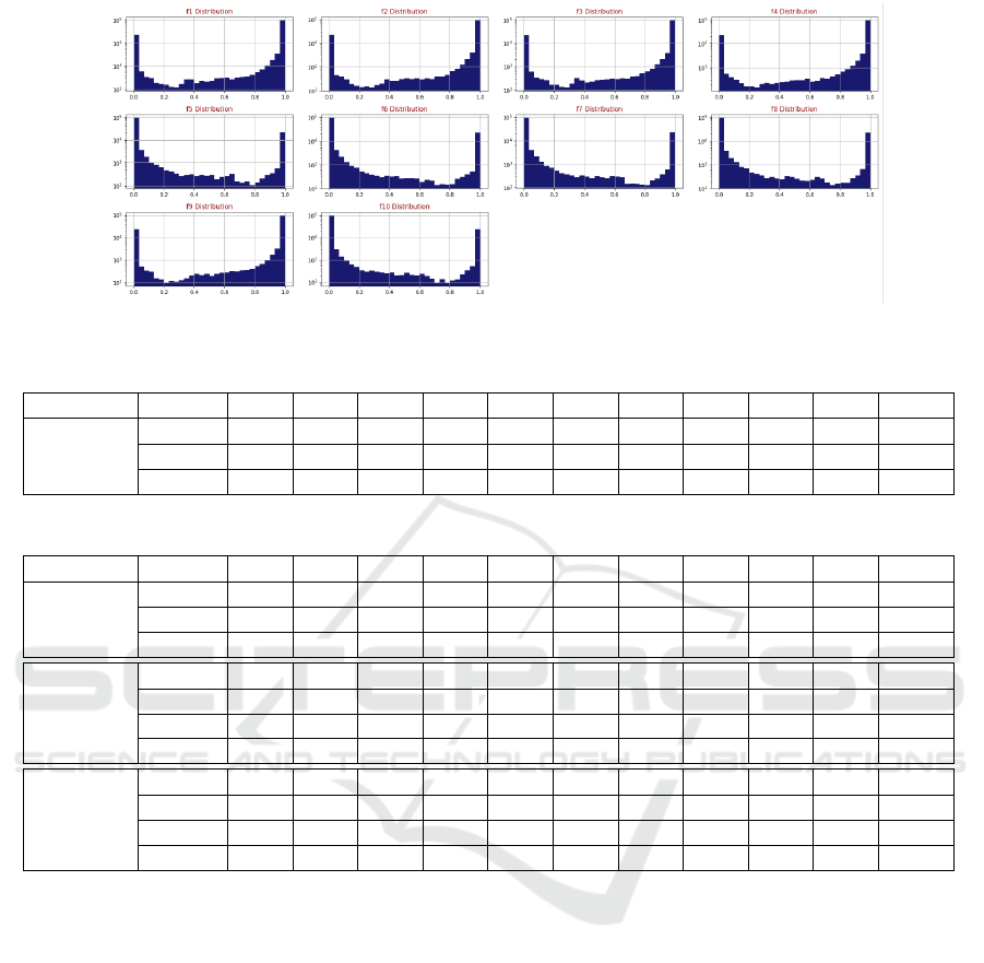
Figure 4: Distribution of the New Features.

Table 2: Training and Testing on Transaction Chunk1.

Classiﬁer Metric #1 #2 #3 #4 #5 #6 #7 #8 #9 #10 Aver.

Initial

Precis 1.00 1.00 1.00 1.00 1.00 1.00 1.00 1.00 1.00 0.99 0.999

Recall 0.87 0.87 0.93 0.84 0.85 0.83 0.84 0.87 0.77 0.84 0.851

F1 0.93 0.93 0.96 0.91 0.92 0.91 0.91 0.93 0.87 0.91 0.918

Table 3: Training and Testing on Transaction Chunk2.

Classiﬁer Metric #1 #2 #3 #4 #5 #6 #7 #8 #9 #10 Aver.

Initial

Precis 1.00 0.99 0.98 0.98 0.99 1.00 0.99 1.00 0.99 0.99 0.991

Recall 0.71 0.77 0.84 0.84 0.81 0.75 0.76 0.85 0.67 0.81 0.781

F1 0.83 0.87 0.90 0.90 0.89 0.86 0.86 0.92 0.80 0.89 0.872

Retrained

Precis 1.00 1.00 1.00 1.00 1.00 1.00 1.00 1.00 1.00 1.00 1.00

Recall 0.70 0.79 0.76 0.82 0.85 0.74 0.84 0.87 0.69 0.66 0.772

F1 0.82 0.88 0.86 0.90 0.92 0.85 0.91 0.93 0.81 0.79 0.867

Time 23s 22s 24s 23s 22s 23s 23s 22s 22s 23s 22.7s

Optimal

Precis 0.97 0.95 0.95 0.96 0.96 0.95 0.95 0.96 0.96 0.96 0.957

Recall 0.86 0.86 0.89 0.88 0.90 0.80 0.90 0.97 0.76 0.88 0.870

F1 0.91 0.90 0.92 0.92 0.93 0.87 0.92 0.96 0.85 0.92 0.910

Time 18s 15s 12s 19s 25s 16s 16s 16s 22s 19s 17.8s

classiﬁer. This expected decrease is due to the higher

number of instances in train chunk1 (60% of data)

than in train chunk2 (40% of data). Therefore, re-

training a model from scratch is not a good solution

(as done in the industry).

3. Optimal Classiﬁer: Lastly, in Table 3, we develop

the ﬁnal optimal model using our IFL algorithm. Us-

ing only one chunk, F1-score of the ﬁnal classiﬁer

improved by 3.8% compared to the initial classiﬁer

(trained on chunk1). Also, Recall, an essential met-

ric in fraud detection, is augmented with 8.9%, which

means we have fewer false negatives with the second

chunk. Moreover, as we are training only the new hid-

den units, the training time is less than the time of the

re-trained classiﬁer. We can conclude that the ﬁnal

classiﬁer outperforms the initial and re-trained classi-

ﬁers using only one chunk.

Another important metric for fraud detection is the

False Negative Rate (FNR), which refers to the rate of

fraudulent transactions detected as normal. Accord-

ing to the average of the ten experiments, the FNR

values of the initial classiﬁer on test chunk1 (called

ICTC1) is 0.149 and on test chunk2 (ICTC2) is

0.219. The FNR of the re-trained classiﬁer (RCTC2)

is 0.228, and FNR of the optimal classiﬁer (OCTC2)

is 0.13. These values demonstrate that the ﬁnal classi-

ﬁer caches more fraudulent cases when fed with new

chunks, reducing FNR over time.

In our point of view, ﬁnancial transactions should

not be stored in a large quantity and for a long time by

the fraud classiﬁers because of conﬁdentiality issues.

In this challenging situation, we train the classiﬁer in-

crementally, chunk by chunk, and discard each chunk

right away. In Table 3, the proposed adaptive learn-

ing algorithm can enhance the performance using one

chunk at a time and with less computational cost.

ICAART 2022 - 14th International Conference on Agents and Artiﬁcial Intelligence

274

6 CONCLUSION

Intending to address the actual behavior of the CCF

detection environment, we introduced a new incre-

mental classiﬁcation algorithm that adjusts gradually

and efﬁciently to new transaction chunks based on

transfer learning and IFL. Transfer learning, which

preserves past knowledge, transforms original fea-

tures into more valuable ones. Then, our adaptive al-

gorithm utilizes them to adapt to subsequent chunks.

IFL extends the network architecture incrementally

by determining the optimal number of hidden units

for each new chunk. Our dynamic learning approach

improves the performance during training without the

necessity of accumulating and storing a large vol-

ume of data and spending too much time on learn-

ing since only the new weights are learned. The pro-

posed approach can be employed on everyday credit

card transactions to prevent the performance from de-

creasing by using current and past knowledge.

REFERENCES

Abdallah, A., Maarof, M. A., and Zainal, A. (2016). Fraud

detection system: A survey. J. Netw. Comput. Appl.,

68:90–113.

Anowar, F. and Sadaoui, S. (2020). Incremental Neural-

Network Learning for Big Fraud Data. In Interna-

tional Conference on Systems, Man, and Cybernetics,

SMC, Toronto, ON, Canada, pages 3551–3557. IEEE.

Anowar, F. and Sadaoui, S. (2021). Incremental Learning

Framework for Real-World Fraud Detection Environ-

ment. Computational Intelligence, 37(1):635–656.

Bayram, B., K

oro

glu, B., and G

onen, M. (2020). Im-

proving Fraud Detection and Concept Drift Adapta-

tion in Credit Card Transactions Using Incremental

Gradient Boosting Trees. In 19th IEEE International

Conference on Machine Learning and Applications

(ICMLA), pages 545–550.

Credit Card Fraud Detection, Anonymized credit card

transactions labeled as fraudulent or genuine (2016).

https://www.kaggle.com/mlg-ulb/creditcardfraud, last

accessed on March 2021.

Credit Card Fraud Statistics In Canada 2021 (2021).

https://www.simplerate.ca/credit-card-fraud-

statistics-canada/, last accessed on May 2021.

Guan, S. U. and Li, S. (2001). Incremental learning with

respect to new incoming input attributes. Neural Pro-

cess. Lett., 14(3):241–260.

Hassan, N., Altiti, O., Ayah, A. A., and Younes, M. (2020).

Credit Card Fraud Detection Based on Machine and

Deep Learning. In 11th International Conference

on Information and Communication Systems (ICICS),

pages 204–208.

Lebichot, B., Paldino, G. M., Bontempi, G., Siblini, W., He-

Guelton, L., and Obl

e, F. (2020). Incremental Learn-

ing Strategies for Credit Cards Fraud Detection: Ex-

tended Abstract. In Webb, G. I., Zhang, Z., Tseng,

V. S., Williams, G., Vlachos, M., and Cao, L., ed-

itors, 7th International Conference on Data Science

and Advanced Analytics, DSAA 2020, Sydney, Aus-

tralia, pages 785–786. IEEE.

Nguyen, T. T., Tahir, H., Abdelrazek, M., and Babar, A.

(2020). Deep Learning Methods for Credit Card Fraud

Detection.

Sadreddin, A. and Sadaoui, S. (2021). Incremental Feature

Learning Using Constructive Neural Networks. In The

33rd IEEE International Conference on Tools with Ar-

tiﬁcial Intelligence (ICTAI), pages 1–5.

Wang, T., Guan, S., Man, K. L., and Ting, T. (2014).

Eeg eye state identiﬁcation using incremental attribute

learning with time-series classiﬁcation. Mathematical

Problems in Engineering, 2014:1–9.

Wang, Y., Wang, L., Yang, F., Di, W., and Chang, Q. (2021).

Advantages of direct input-to-output connections in

neural networks: The elman network for stock index

forecasting. Inf. Sci., 547:1066–1079.

Weiss, K., Khoshgoftaar, T. M., and Wang, D. (2016). A

survey of transfer learning. Journal of Big Data,

3(1):1–40.

Worldwide Credit Card Fraud Statistics 2019 (2020).

https://nilsonreport.com

/content

promo.php?id promo=16/, last accessed on

June 2021.

Incremental Feature Learning for Fraud Data Stream

275